Advanced Mathematics and Mechanics Applications Using MATLAB phần 2 ppt

176: R2=[real(u2);imag(u2);z2];
177:
178:
% Get curve properties from crvprp3d
179: [T,N,B,kappa]=crvprp3d(R1,R2);
180:
181:
%==============================================
182:
183:
function val=splined(xd,yd,x,if2)
184: %
185: % val=splined(xd,yd,x,if2)
186: % ~~~~~~~~~~~~~~~~~~~~~~~~
187: %
188: % This function evaluates the first or second
189: % derivative of the piecewise cubic
190: % interpolation curve defined by the intrinsic
191: % function spline provided in MATLAB.If fewer
192: % than four data points are input, then simple
193: % polynomial interpolation is employed
194: %
195: % xd,yd - data vectors determining the spline
196: % curve produced by function spline
197: % x - vector of values where the first or
198: % the second derivative are desired
199: % if2 - a parameter which is input only if
200: % y’’(x) is required. Otherwise, y’(x)
201: % is returned.
202: %
203: % val - the first or second derivative values

204: % for the spline
205: %
206: % User m functions called: none
207:
208:
n=length(xd); [b,c]=unmkpp(spline(xd,yd));
209: if n>3 % Use a cubic spline
210: if nargin==3, c=[3*c(:,1),2*c(:,2),c(:,3)];
211: else, c=[6*c(:,1),2*c(:,2)]; end
212: val=ppval(mkpp(b,c),x);
213: else % Use a simple polynomial
214: c=polyder(polyfit(xd(:),yd(:),n-1));
215: if nargin==4, c=polyder(c); end
216: val=polyval(c,x);
217: end
218:
219:
%=================================================
220:
© 2003 by CRC Press LLC
221: % function range=cubrange(xyz,ovrsiz)
222: % See Appendix B
2.8.2 Surface Properties
Surfaces are two-dimensional regions described parametrically as
R(u, v)=
ˆ
ıx(u, v)+
ˆ
u(u, v)+
ˆ

kz(u, v)
where u and v are scalar parameters. This parametric form is helpful for generating a
grid of points on the surface as well as for computing surface tangents and the surface
normal. Holding v Þxed while u varies generates a curve in the surface called a u
coordinate line. A tangent vector to the u-line is given by
g
u
=
∂R
∂u
=
ˆ
ı
∂x
∂u
+
ˆ

∂y
∂u
+
ˆ
k
∂z
∂u
.
Similarly, holding u Þxed and varying v produces a v-line with tangent vector
g
v
=

∂R
∂v
=
ˆ
ı
∂x
∂v
+
ˆ

∂y
∂v
+
ˆ
k
∂z
∂v
.
Consider the following cross product.
g
u
× g
v
du dv =ˆndS.
In this equation ˆn is the unit surface normal and dS is the area of a parallelogram
shaped surface element having sides deÞned by g
u
du and g
v
dv.

The intrinsic functions surf(X,Y,Z) and mesh(X,Y,Z) depict surfaces by showing
a grid network and related surface patches characterized when parameters u and v
are varied over constant limits. Thus, values
(u
ı
,v

) , 1 ≤ ı ≤ n, 1 ≤  ≤ m
lead to matrices
X =[x(u
ı
,v

)] ,Y=[y(u
ı
,v

)] ,Z=[z(u
ı
,v

)]
from which surface plots are obtained. Function surf colors the surface patches
whereas mesh colors the grid lines.
As a simple example, consider the ellipsoidal surface described parametrically as
x = a cos θ cos φ, y= b cos θ sin φ, z= c sin θ
where −
π
2
≤ θ ≤

π
2
, −π ≤ φ ≤ π. The surface equation evidently satisÞes the
familiar equation

x
a

2
+

y
b

2
+

z
c

2
=1
© 2003 by CRC Press LLC
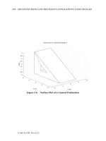
for an ellipsoid. The function elipsoid(a,b,c) called with a =2, b =1.5, c =1
produces the surface plot in Figure 2.18.
Many types of surfaces can be parameterized in a manner similar to the ellipsoid.
We will examine two more problems involving a torus and a conical frustum. Con-
sider a circle of radius b lying in the xz-plane with its center at [a,0,0]. Rotating
the circle about the z-axis produces a torus having the surface equation
x =[a + b cos θ]cosφ, y=[a + b cos θ] , sin φ, z= b sin φ

where −π ≤ θ ≤ π, −π ≤ φ ≤ π.
This type of equation is used below in an example involving several bodies. Let
us also produce a surface covering the ends and side of a conical frustum (a cone
with the top cut off). The frustum has base radius r
b
, top radius r
t
, and height h,
with the symmetry axis along the z-axis. The surface can be parameterized using an
azimuthal angle θ and an arc length parameter relating to the axial direction. The
lateral side length is
r
s
=

h
2
+(r
b
− r
t
)
2
.
Let us take 0 ≤ s ≤ (r
b
+ r
s
+ r
t

) and describe the surface R(s, θ) by coordinate
functions
x = r(s)cosθ, y= r(s)sinθ, z= z(s)
where 0 ≤ θ ≤ 2π and
r(s)=s, 0 ≤ s ≤ r
b
r(s)=r
b
+
(r
t
− r
b
)(s −r
b
)
r
s
,z=
h(s − r
b
)
r
s
,r
b
≤ s ≤ (r
b
+ r
s

)
r(s)=r
b
+ r
s
+ r
t
− r,z= h, (r
b
+ r
s
) ≤ s ≤ (r
b
+ r
s
+ r
t
) .
The function frus produces a grid of points on the surface in terms of r
b
, r
t
, h, the
number of increments on the base, the number of increments on the side, and the
number of increments on the top. Figure 2.16 shows the plot generated by frus.
An example called srfex employs the ideas just discussed and illustrates how
MATLAB represents several interesting surfaces. Points on the surface of an an-
nulus symmetric about the z-axis are created, and two more annuli are created by
interchanging axes. A pyramid with a square base is also created and the combina-
tion of four surfaces is plotted by Þnding a data range to include all points and then

plotting each surface in succession using the hold instruction (See Figure 2.16). Al-
though the rendering of surface intersections is not perfect, a useful description of a
fairly involved geometry results. Combined plotting of several intersecting surfaces
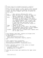
is implemented in a general purpose function surfmany. The default data case for
surfmany produces the six=legged geometry shown in Figure 2.17.
This section is concluded with a discussion of how a set of coordinate points can
be moved to a new position by translation and rotation of axes. Suppose a vector
r =
ˆ
ıx +
ˆ
y +
ˆ
kz
© 2003 by CRC Press LLC
Spike and Intersecting Toruses
Figure 2.16: Spike and Intersecting Toruses
undergoes a coordinate change which moves the initial coordinate origin to (X
o
,Y
o
,Z
o
)
and moves the base vectors
ˆ
ı,
ˆ
,
ˆ

k into ˆe
1
, ˆe
2
, ˆe
3
. Then the endpoint of r passes to
R =
ˆ
ıX +
ˆ
Y +
ˆ
kZ = R
o
+ˆe
1
x +ˆe
2
y +ˆe
3
z
where
R
o
=
ˆ
ıX
o
+

ˆ
Y
o
+
ˆ
kZ
o
.
Let us specify the directions of the new base vectors by employing the columns of a
matrix V where we take
ˆe
3
=
V (:, 1)
norm[V (:, 1)]
.
If V (:, 2) exists we take V (:, 1) × V (:, 2) and unitize this vector to produce ˆe
2
. The
triad is completed by taking ˆe
1
=ˆe
2
× ˆe
3
. In the event that V (:, 2) is not provided,
we use [1;0;0] and proceed as before. The functions rgdbodmo and rotatran
can be used to transform points in the manner described above.
© 2003 by CRC Press LLC
−5

0
5
−5
0
5
−8
−6
−4
−2
0
2
4
6
8
x axis
SEVERAL SURFACES COMBINED
y axis
z axis
Figure 2.17: Surface With Six Legs
© 2003 by CRC Press LLC
2
2.5
3
3.5
4
3
3.5
4
4.5
5

4
4.5
5
5.5
6
x axis
ROTATED AND TRANSLATED ELLIPSOID
y axis
z axis
Figure 2.18: Rotated and Translated Ellipsoid Surfaces
© 2003 by CRC Press LLC
2.8.3 Program Output and Code
Function srfex
1: function [x1,y1,x2,y2,x3,y3,xf,yf,zf]=
2: srfex(da,na,df,nf)
3: % [x1,y1,x2,y2,x3,y3,xf,yf,zf]=
4: % srfex(da,na,df,nf)
5: % ~~~~~~~~~~~~~~~~~~~~~~~~~~~~~~~~~~~~~~~~~~~~~
6: %
7: % This graphics example draws three toruses
8: % intersecting a spike.
9: %
10: % User m functions called: frus, surfmany
11:
12:
if nargin==0
13: da=[4.0,.45]; na=[42,15];
14: df=[2.2,0,15]; nf=[43,4];
15: end
16:

17:
% Create a torus with polygonal cross section.
18: % Data for the torus is stored in da and na
19:
20:
r0=da(1); r1=da(2); nfaces=na(1); nlat=na(2);
21: t=linspace(0,2*pi,nlat)’;
22: xz=[r0+r1*cos(t),r1*sin(t)];
23: z1=xz(:,2); z1=z1(:,ones(1,nfaces+1));
24: th=linspace(0,2*pi,nfaces+1);
25: x1=xz(:,1)*cos(th); y1=xz(:,1)*sin(th);
26: y2=x1; z2=y1; x2=z1; y3=x2; z3=y2; x3=z2;
27:
28:
% Create a frustum of a pyramid. Data for the
29: % frustum is stored in df and nf
30: rb=df(1); rt=df(2); h=df(3);
31: [xf,yf,zf]=frus(rb,rt,h,nf); zf=zf 35*h;
32:
33:
% Plot four figures combined together
34: hold off; clf; close;
35: surfmany(x1,y1,z1,x2,y2,z2,x3,y3,z3,xf,yf,zf)
36: xlabel(’x axis’); ylabel(’y axis’);
37: zlabel(’z axis’);
38: title(’Spike and Intersecting Toruses’);
39: axis equal; axis(’off’);
40: colormap([1 1 1]); figure(gcf); hold off;
© 2003 by CRC Press LLC
41: % print -deps srfex

42:
43:
%=============================================
44:
45:
function [X,Y,Z]=frus(rb,rt,h,n,noplot)
46: %
47: % [X,Y,Z]=frus(rb,rt,h,n,noplot)
48: % ~~~~~~~~~~~~~~~~~~~~~~~~~~~~~~
49: %
50: % This function computes points on the surface
51: % of a conical frustum which has its axis along
52: % the z axis.
53: %
54: % rb,rt,h - the base radius,top radius and
55: % height
56: % n - vector of two integers defining the
57: % axial and circumferential grid
58: % increments on the surface
59: % noplot - parameter input when no plot is
60: % desired
61: %
62: % X,Y,Z - points on the surface
63: %
64: % User m functions called: none
65:
66:
if nargin==0
67: rb=2; rt=1; h=3; n=[23, 35];
68: end

69:
70:
th=linspace(0,2*pi,n(2)+1)’-pi/n(2);
71: sl=sqrt(h^2+(rb-rt)^2); s=sl+rb+rt;
72: m=ceil(n(1)/s*[rb,sl,rt]);
73: rbot=linspace(0,rb,m(1));
74: rside=linspace(rb,rt,m(2));
75: rtop=linspace(rt,0,m(3));
76: r=[rbot,rside(2:end),rtop(2:end)];
77: hbot=zeros(1,m(1));
78: hside=linspace(0,h,m(2));
79: htop=h*ones(1,m(3));
80: H=[hbot,hside(2:end),htop(2:end)];
81: Z=repmat(H,n(2)+1,1);
82: xy=exp(i*th)*r; X=real(xy); Y=imag(xy);
83: if nargin<5
84: surf(X,Y,Z); title(’Frustum’); xlabel(’x axis’)
85: ylabel(’y axis’), zlabel(’z axis’)
© 2003 by CRC Press LLC
86: grid on, colormap([1 1 1]);
87: figure(gcf);
88: end
89:
90:
%=============================================
91:
92:
function surfmany(varargin)
93: %function surfmany(x1,y1,z1,x2,y2,z2,
94: % x3,y3,z3, ,xn,yn,zn)

95: % This function plots any number of surfaces
96: % on the same set of axes without shape
97: % distortion. When no input is given then a
98: % six-legged solid composed of spheres and
99: % cylinders is shown.
100: %
101: % User m functions called: none
102: %
103:
104:
if nargin==0
105: % Default data for a six-legged solid
106: n=10; rs=.25; d=7; rs=2; rc=.75;
107: [xs,ys,zs]=sphere; [xc,yc,zc]=cylinder;
108: xs=rs*xs; ys=rs*ys; zs=rs*zs;
109: xc=rc*xc; yc=rc*yc; zc=2*d*zc-d;
110: x1=xs; y1=ys; z1=zs;
111: x2=zs+d; y2=ys; z2=xs;
112: x3=zs-d; y3=ys; z3=xs;
113: x4=xs; y4=zs-d; z4=ys;
114: x5=xs; y5=zs+d; z5=ys;
115: x6=xs; y6=ys; z6=zs+d;
116: x7=xs; y7=ys; z7=zs-d;
117: x8=xc; y8=yc; z8=zc;
118: x9=zc; y9=xc; z9=yc;
119: x10=yc; y10=zc; z10=xc;
120: varargin={x1,y1,z1,x2,y2,z2,x3,y3,z3,
121: x4,y4,z4,x5,y5,z5,x6,y6,z6,x7,y7,z7,
122: x8,y8,z8,x9,y9,z9,x10,y10,z10};
123: end

124:
125:
% Find the data range
126: n=length(varargin);
127: r=realmax*[1,-1,1,-1,1,-1];
128: s=inline(’min([a;b])’,’a’,’b’);
129: b=inline(’max([a;b])’,’a’,’b’);
130: for k=1:3:n
© 2003 by CRC Press LLC
131: x=varargin{k}; y=varargin{k+1};
132: z=varargin{k+2};
133: x=x(:); y=y(:); z=z(:);
134: r(1)=s(r(1),x); r(2)=b(r(2),x);
135: r(3)=s(r(3),y); r(4)=b(r(4),y);
136: r(5)=s(r(5),z); r(6)=b(r(6),z);
137: end
138:
139:
% Plot each surface
140: hold off, newplot
141: for k=1:3:n
142: x=varargin{k}; y=varargin{k+1};
143: z=varargin{k+2};
144: surf(x,y,z); axis(r), hold on
145: end
146:
147:
% Set axes and display the combined plot
148: axis equal, axis(r), grid on
149: xlabel(’x axis’), ylabel(’y axis’)

150: zlabel(’z axis’)
151: title(’SEVERAL SURFACES COMBINED’)
152: % colormap([127/255 1 212/255]); % aquamarine
153: colormap([1 1 1]);, figure(gcf), hold off
Function rgdbodmo
1: function [X,Y,Z]=rgdbodmo(x,y,z,v,R0)
2: %
3: % [X,Y,Z]=rgdbodmo(x,y,z,v,R0)
4: % ~~~~~~~~~~~~~~~~~~~~~~~~~~~~
5: %
6: % This function transforms coordinates x,y,z to
7: % new coordinates X,Y,Z by rotating and
8: % translating the reference frames. When no
9: % input is given, an example involving an
10: % ellipsoid is run.
11: %
12: % x,y,z - initial coordinate matrices referred
13: % to base vectors [1;0;0], [0;1;0] and
14: % [0;0;1]. Columns of v are used to
15: % create new basis vectors i,j,k such
16: % that a typical point [a;b;c] is
17: % transformed into [A;B;C] according
18: % to the equation
© 2003 by CRC Press LLC
19: % [A;B;C]=R0(:)+[i,j,k]*[a;b;c]
20: % v - a matrix having three rows and either
21: % one or two columns used to construct
22: % the new basis [i,j,k] according to
23: % methods employed function rotatran
24: % R0 - a vector which translates the rotated

25: % coordinates when R0 is input.
26: % Otherwise no translation is imposed.
27: %
28: % X,Y,Z - matrices containing the transformed
29: % coordinates
30: %
31: % User m functions called: elipsoid, rotatran
32:
33:
if nargin==0
34: [x,y,z]=elipsoid(1,1,2,[17,33],0);R0=[3;4;5];
35: v=[[1;1;1],[1;1;0]];
36: end
37: [n,m]=size(x); XYZ=[x(:),y(:),z(:)]*rotatran(v)’;
38: X=XYZ(:,1); Y=XYZ(:,2); Z=XYZ(:,3);
39: if ~isempty(R0)
40: X=X+R0(1); Y=Y+R0(2); Z=Z+R0(3);
41: end
42: X=reshape(X,n,m); Y=reshape(Y,n,m);
43: Z=reshape(Z,n,m);
44: if nargin==0
45: close; surf(X,Y,Z), axis equal, grid on
46: title(’ROTATED AND TRANSLATED ELLIPSOID’)
47: xlabel(’x axis’), ylabel(’y axis’)
48: zlabel(’z axis’),colormap([1 1 1]); shg
49: end
50:
51:
%==============================================
52:

53:
function [x,y,z]=elipsoid(a,b,c,n,noplot)
54: %
55: % [x,y,z]=elipsoid(a,b,c,n,noplot)
56: % ~~~~~~~~~~~~~~~~~~~~~~~~~~~~~~~
57: % This function plots an ellipsoid having semi-
58: % diameters a,b,c
59: % a,b,c - semidiameters of the ellipsoid defined
60: % by (x/a)^2+(y/b)^2+(z/c)^2=1
61: % n - vector [nth,nph] giving the number of
62: % theta values and phi values used to plot
63: % the surface
© 2003 by CRC Press LLC
64: % noplot - omit this parameter if no plot is desired
65: % x,y,z - matrices of points on the surface
66: %
67: % User m functions called: none
68: %
69:
70:
if nargin==0, a=2; b=1.5; c=1; n=[17,33]; end
71: nth=n(1); nph=n(2);
72: th=linspace(-pi/2,pi/2,nth)’; ph=linspace(-pi,pi,nph);
73: x=a*cos(th)*cos(ph); y=b*cos(th)*sin(ph);
74: z=c*sin(th)*ones(size(ph));
75: if nargin<5
76: surf(x,y,z); axis equal
77: title(’ELLIPSOID’), xlabel(’x axis’)
78: ylabel(’y axis’), zlabel(’z axis’)
79: colormap([1 1 1]); grid on, figure(gcf)

80: end
81:
82:
%==============================================
83:
84:
function mat=rotatran(v)
85: %
86: % mat=rotatran(v)
87: % ~~~~~~~~~~~~~~~
88: % This function creates a rotation matrix based
89: % on the columns of v.
90: %
91: % v - a matrix having three rows and either
92: % one or two columns which are used to
93: % create an orthonormal triad [i,j,k]
94: % returned in the columns of mat. The
95: % third base vector k is defined as
96: % v(:,1)/norm(v(:,1)). If v has two
97: % columns then, v(:,1) and v(:,2) define
98: % the xz plane with the direction of j
99: % defined by cross(v(:,1),v(:2)). If only
100: % v(:,1) is input, then v(:,2) is set
101: % to [1;0;0].
102: %
103: % mat - the matrix having columns containing
104: % the basis vectors [i,j,k]
105: %
106: % User m functions called: none
107: %

108:
© 2003 by CRC Press LLC
109: k=v(:,1)/norm(v(:,1));
110: if size(v,2)==2, p=v(:,2); else, p=[1;0;0]; end
111: j=cross(k,p); nj=norm(j);
112: if nj~=0
113: j=j/nj; mat=[cross(j,k),j,k];
114: else
115: mat=[[0;1;0],cross(k,[0;1;0]),k];
116: end
© 2003 by CRC Press LLC
Chapter 3
SummaryofConceptsfromLinearAlgebra
3.1 Introduction
This chapter brießy reviews important concepts of linear algebra. We assume the
reader already has some experience working with matrices, and linear algebra ap-
plied to solving simultaneous equations and eigenvalue problems. MATLAB has ex-
cellent capabilities to perform matrix operations using the fastest and most accurate
algorithms currently available. The books by Strang [96] and Golub and Van Loan
[47] give comprehensive treatments of matrix theory and of algorithm developments
accounting for effects of Þnite precision arithmetic. One beautiful aspect of matrix
theory is that fairly difÞcult proofs often lead to remarkably simple results valuable
to users not necessarily familiar with all of the theoretical developments. For in-
stance, the property that every real symmetric matrix of order n has real eigenvalues
and a set of n orthonormal eigenvectors can be understood and used by someone
unfamiliar with the proof. The current chapter summarizes a number of fundamen-
tal matrix properties and some of the related MATLAB functions. The intrinsic
matrix functions use highly efÞcient algorithms originally from the LINPACK and
EISPACK libraries which have now been superceded by LAPACK. [34, 42, 89]. Dr.
Cleve Moler, the Chairman and Chief Scientist at The MathWorks, contributed to

development of these systems. He also wrote the Þrst version of MATLAB. Readers
should simultaneously study the current chapter and the MATLAB demo program
on linear algebra.
3.2 Vectors, Norms, Linear Independence, and Rank
Consider an n by m matrix
A =[a
ı
] , 1 ≤ ı ≤ n, 1 ≤  ≤ m,
having real or complex elements. The shape of a matrix is computed by size(A)
which returns a vector containing n and m. The matrix obtained by conjugating
the matrix elements and interchanging columns and rows is called the transpose.
© 2003 by CRC Press LLC
Transposition is accomplished with a

operator, so that
A
transpose = A

.
Transposition without conjugation of the elements can be performed as A.

or as
conj(A

). Of course, whenever A is real, A

is simply the traditional transpose.
The structure of a matrix A is characterized by the matrix rank and sets of basis
vectors spanning four fundamental subspaces. The rank r is the maximum number
of linearly independent rows or columns in the matrix. We discuss these spaces in

the context of real matrices. The basic subspaces are:
1. The column space containing all vectors representable as a linear combination
of the columns of A. The column space is also referred to as the range or the
span.
2. The null space consisting of all vectors perpendicular to every row of A.
3. The row space consisting of all vectors which are linear combinations of the
rows of A.
4. The left null space consisting of all vectors perpendicular to every column of
A.
MATLAB has intrinsic functions to compute rank and subspace bases
• matrix
rank = rank(A)
• column
space = orth(A)
• null
space = null(A)
• row
space = orth(A

)

• left null space = null(A

)

The basis vectors produced by null and orth are orthonormal. They are generated
using the singular value decomposition algorithm [47]. The MATLAB function to
perform this type of computation is named svd.
3.3 Systems of Linear Equations, Consistency, and Least Squares
Approximation

Let us discuss the problem of solving systems of simultaneous equations. Repre-
senting a vector B as a linear combination of the columns of A requires determina-
tion of a vector X to satisfy
AX = B ⇐⇒
m

=1
A(:,) x()=B
© 2003 by CRC Press LLC
where the ’th column of A is scaled by the ’th component of X to form the lin-
ear combination. The desired representation is possible if and only if B lies in the
column space of A. This implies the consistency requirement that A and [A, B]
must have the same rank. Even when a system is consistent, the solution will not be
unique unless all columns of A are independent. When matrix A, with n rows and m
columns, has rank r less than m, the general solution of AX = B is expressible as
any particular solution plus an arbitrary linear combination of m − r vectors form-
ing a basis for the null space. MATLAB gives the solution vector as X = A\ B.
When r is less than m, MATLAB produces a least squares solution having as many
components as possible set equal to zero.
In instances where the system is inconsistent, regardless of how X is chosen, the
error vector deÞned by
E = AX − B
can never be zero. An approximate solution can be obtained by making E normal to
the columns of A. We get
A

AX = A

B
which is known as the system of normal equations. They are also referred to as least

squares error equations. It is not difÞcult to show that the same equations result by
requiring E to have minimum length. The normal equations are always consistent
and are uniquely solvable when rank(A)=m. A comprehensive discussion of least
squares approximation and methods for solving overdetermined systems is presented
by Lawson and Hanson [62]. It is instructive to examine the results obtained from
the normal equations when A is square and nonsingular. The least squares solution
would give
X =(A

A)
−1
A

B = A
−1
(A

)
−1
A

B = A
−1
B.
Therefore, the least squares solution simply reduces to the exact solution of AX = B
for a consistent system. MATLAB handles both consistent and inconsistent systems
as X = A\B. However, it is only sensible to use the least squares solution of an
inconsistent system when AX produces an acceptable approximation to B. This
implies
norm(AX − B) <tol∗norm(B)

where tol is suitably small.
A simple but important application of overdetermined systems arises in curve Þt-
ting. An equation of the form
y(x)=
m

=1
f

(x)c

involving known functions f

(x), such as x
−1
for polynomials, must approximately
match data values (X
ı
,Y
ı
), 1 ≤ ı ≤ n, with n>m. We simply write an overdeter-
mined system
n

=1
f

(X
ı
)c


≈ Y
ı
, 1 ≤ ı ≤ n
© 2003 by CRC Press LLC
and obtain the least squares solution. The approximation is acceptable if the error
components
e
ı
=
m

=1
f

(X
ı
)c

− Y
ı
are small enough and the function y(x) is also acceptably smooth between the data
points.
Let us illustrate how well MATLAB handles simultaneous equations by construct-
ing the steady-state solution of the matrix differential equation
M ¨x + C ˙x + Kx = F
1
cos(ωt)+F
2
sin(ωt)

where M , C, and K are constant matrices and F
1
and F
2
are constant vectors. The
steady-state solution has the form
x = X
1
cos(ωt)+X
2
sin(ωt)
where X
1
and X
2
are chosen so that the differential equation is satisÞed. Evidently
˙x = −ωX
1
sin(ωt)+ωX
2
cos(ωt)
and
¨x = −ω
2
x.
Substituting the assumed form into the differential equation and comparing sine and
cosine terms on both sides yields
(K − ω
2
M)X

1
+ ωCX
2
= F
1
,
−ωCX
1
+(K − ω
2
M)X
2
= F
2
.
The equivalent partitioned matrix is

(K − ω
2
M) ωC
−ωC (K − ω
2
M)

X
1
X
2

=


F
1
F
2

.
A simple MATLAB function to produce X
1
and X
2
when M, C, K, F
1
, F
2
, and ω
are known is
function [x1,x2,xmax]=forcresp(m,c,k,f1,f2,w)
kwm=k-(w*w)*m; wc=w*c;
x=[kwm,wc;-wc,kwm]\[f1;f2]; n=length(f1);
x1=x(1:n); x2=x(n+1:2*n);
xmax=sqrt(x1.*x1+x2.*x2);
The vector, xmax,deÞned in the last line of the function above, has components
specifying the maximum amplitude of each component of the steady-state solution.
© 2003 by CRC Press LLC
The main computation in this function occurs in the third line, where matrix concate-
nation is employed to form a system of 2n equations with x being the concatenation
of X
1
and X

2
. The fourth line uses vector indexing to extract X
1
and X
2
from x.
The notational simplicity of MATLAB is elegantly illustrated by these features: a)
any required temporary storage is assigned and released dynamically, b) no looping
operations are needed, c) matrix concatenation and inversion are accomplished with
intrinsic functions using matrices and vectors as sub-elements of other matrices, and
d) extraction of sub-vectors is accomplished by use of vector indices. The impor-
tant differential equation just discussed will be studied further in Article 3.5.3 where
eigenvalues and complex arithmetic are used to obtain a general solution satisfying
arbitrary initial conditions.
3.4 Applications of Least Squares Approximation
The idea of solving an inconsistent system of equations in the least squares sense,
so that some required condition is approximately satisÞed, has numerous applica-
tions. Typically, we are dealing with a large number of equations (several hundred
is common) involving a smaller number of parameters used to closely Þt some con-
straint. Linear boundary value problems often require the solution of a differential
equation applicable in the interior of a region while the function values are known on
the boundary. This type of problem can sometimes be handled by using a series of
functions which satisfy the differential equation exactly. Weighting the component
solutions to approximately match the remaining boundary condition may lead to use-
ful results. Below, we examine three instances where least squares approximation is
helpful.
3.4.1 A Membrane Deßection Problem
Let us illustrate how least squares approximation can be used to compute the trans-
verse deßection of a membrane subjected to uniform pressure. The transverse de-
ßection u for a membrane which has zero deßection on a boundary L satisÞes the

differential equation
∂
2
u
∂x
2
+
∂
2
u
∂y
2
= −γ,(x,y) inside L
where γ is a physical constant. Properties of harmonic functions [18] imply that the
differential equation is satisÞed by a series of the form
u = γ

−|z|
2
4
+
n

=1
c

real(z
−1
)


© 2003 by CRC Press LLC
−0.8
−0.6
−0.4
−0.2
0
0.2
0.4
0.6
0.8
1
−1
−0.5
0
0.5
1
−0.05
0
0.05
0.1
0.15
0.2
0.25
0.3
Membrane Deflection
x axis
y axis
deflection
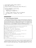
Figure 3.1: Surface Plot of Membrane
where z = x + ıy and constants c


are chosen to make the boundary deßection as
small as possible, in the least squares sense. As a speciÞc example, we analyze a
membrane consisting of a rectangular part on the left joined with a semicircular part
on the right. The surface plot in Figure 3.1 and the contour plot in Figure 3.2 were
produced by the function membran listed below. This function generates boundary
data, solves for the series coefÞcients, and constructs plots depicting the deßection
pattern. The results obtained using a twenty-term series satisfy the boundary condi-
tions quite well.
© 2003 by CRC Press LLC
−1 −0.5 0 0.5 1
−1
−0.8
−0.6
−0.4
−0.2
0
0.2
0.4
0.6
0.8
1
x axis
y axis
Membrane Surface Contour Lines
Figure 3.2: Membrane Surface Contour Lines
© 2003 by CRC Press LLC
MATLAB Example
Function membran
1: function [dfl,cof]=membran(h,np,ns,nx,ny)

2: % [dfl,cof]=membran(h,np,ns,nx,ny)
3: % ~~~~~~~~~~~~~~~~~~~~~~~~~~~~~~~~
4: % This function computes the transverse
5: % deflection of a uniformly tensioned membrane
6: % which is subjected to uniform pressure. The
7: % membrane shape is a rectangle of width h and
8: % height two joined with a semicircle of
9: % diameter two.
10: %
11: % Example use: membran(0.75,100,50,40,40);
12: %
13: % h - the width of the rectangular part
14: % np - the number of least square points
15: % used to match the boundary
16: % conditions in the least square
17: % sense is about 3.5*np
18: % ns - the number of terms used in the
19: % approximating series to evaluate
20: % deflections. The series has the
21: % form
22: %
23: % dfl = abs(z)^2/4 +
24: % sum({j=1:ns},cof(j)*
25: % real(z^(j-1)))
26: %
27: % nx,ny - the number of x points and y points
28: % used to compute deflection values
29: % on a rectangular grid
30: % dfl - computed array of deflection values
31: % cof - coefficients in the series

32: % approximation
33: %
34: % User m functions called: none
35:
36:
if nargin==0
37: h=.75; np=100; ns=50; nx=40; ny=40;
38: end
39:
40:
% Generate boundary points for least square
© 2003 by CRC Press LLC
41: % approximation
42: z=[exp(i*linspace(0,pi/2,round(1.5*np))),
43: linspace(i,-h+i,np),
44: linspace(-h+i,-h,round(np/2))];
45: z=z(:); xb=real(z); xb=[xb;xb(end:-1:1)];
46: yb=imag(z); yb=[yb;-yb(end:-1:1)]; nb=length(xb);
47:
48:
% Form the least square equations and solve
49: % for series coefficients
50: a=ones(length(z),ns);
51: for j=2:ns, a(:,j)=a(:,j-1).*z; end
52: cof=real(a)\(z.*conj(z))/4;
53:
54:
% Generate a rectangular grid for evaluation
55: % of deflections
56: xv=linspace(-h,1,nx); yv=linspace(-1,1,ny);

57: [x,y]=meshgrid(xv,yv); z=x+i*y;
58:
59:
% Evaluate the deflection series on the grid
60: dfl=-z.*conj(z)/4+
61: real(polyval(cof(ns:-1:1),z));
62:
63:
% Set values outside the physical region of
64: % interest to zero
65: dfl=real(dfl).*(1-((abs(z)>=1)&(real(z)>=0)));
66:
67:
% Make surface and contour plots
68: hold off; close; surf(x,y,dfl);
69: xlabel(’x axis’); ylabel(’y axis’);
70: zlabel(’deflection’); view(-10,30);
71: title(’Membrane Deflection’); colormap([1 1 1]);
72: shg, disp(
73: ’Press [Enter] to show a contour plot’), pause
74: % print -deps membdefl;
75: contour(x,y,dfl,15,’k’); hold on
76: plot(xb,yb,’k-’); axis(’equal’), hold off
77: xlabel(’x axis’); ylabel(’y axis’);
78: title(’Membrane Surface Contour Lines’), shg
79: % print -deps membcntr
© 2003 by CRC Press LLC
3.4.2 Mixed Boundary Value Problem for a Function Harmonic Inside
a Circular Disk
Problems where a partial differential equation is to be solved inside a region with

certain conditions imposed on the boundary occur in many situations. Often the dif-
ferential equation is solvable exactly in a series form containing arbitrary linear com-
binations of known functions. An approximation procedure imposing the boundary
conditions to compute the series coefÞcients produces a satisfactory solution if the
desired boundary conditions are found to be well satisÞed. Consider a mixed bound-
ary value problem in potential theory [73] pertaining to a circular disk of unit radius.
We seek u(r, θ) where function values are speciÞed on one part of the boundary
and normal derivative values are speciÞed on the remaining part. The mathematical
formulation is
∂
2
u
∂r
2
+
1
r
∂u
∂r
+
1
r
2
∂
2
u
∂θ
2
=0, 0 ≤ r<1 , 0 ≤ θ ≤ 2π,
u(1,θ)=f (θ) , −α<θ<α,

∂u
∂r
(1,θ)=g(θ) ,α<θ<2π − α.
The differential equation has a series solution of the form
u(r, θ)=c
0
+
∞

n=1
r
n
[c
n
cos(nθ)+d
n
sin(nθ)]
where the boundary conditions require
c
0
+
∞

n=1
[c
n
cos(nθ)+d
n
sin(nθ)] = f (θ) , −α<θ<α,
and

∞

n=1
n[c
n
cos(nθ)+d
n
sin(nθ)] = g(θ) ,α<θ<2π − α.
The series coefÞcients can be obtained by least squares approximation. Let us ex-
plore the utility of this approach by considering a particular problem for a Þeld which
is symmetric about the x-axis. We want to solve
∇
2
u =0,r<1,
u(1,θ)=cos(θ) , |θ| <π/2,
∂u
∂r
(1,θ)=0,π/2 < |θ|≤π.
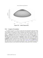
This problem characterizes steady-state heat conduction in a cylinder with the left
half insulated and the right half held at a known temperature. The appropriate series
solution is
u =
∞

n=0
c
n
r
n
cos(nθ)

© 2003 by CRC Press LLC
subject to
∞

n=0
c
n
cos(nθ)=cos(θ) for |θ| <π/2,
and
∞

n=0
nc
n
cos(nθ)=0for π/2 < |θ|≤π.
We solve the problem by truncating the series after a hundred or so terms and forming
an overdetermined system derived by imposition of both boundary conditions. The
success of this procedure depends on the series converging rapidly enough so that a
system of least squares equations having reasonable order and satisfactory numerical
condition results. It can be shown by complex variable methods (see Muskhelishvili
[73]) that the exact solution of our problem is given by
u = real

z + z
−1
+(1− z
−1
)

z

2
+1

/2 , |z|≤1
where the square root is deÞned for a branch cut along the right half of the unit circle
with the chosen branch being that which equals +1 at z =0. Readers familiar with
analytic function theory can verify that the boundary values of u yield
u(1,θ)=cos(θ) , |θ|≤π/2,
u(1,θ)=cos(θ)+sin(|θ|/2)

2|cos(θ)| ,π/2 ≤|θ|≤π.
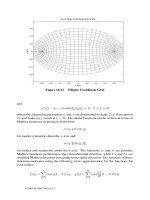
A least squares solution is presented in function mbvp. Results from a series of
100 terms are shown in Figure 3.3. The series solution is accurate within about one
percent error except for points near θ = π/2. Although the results are not shown
here, using 300 terms gives a solution error nowhere exceeding 4 percent. Hence
the least squares series solution provides a reasonable method to handle the mixed
boundary value problem.
© 2003 by CRC Press LLC
0 20 40 60 80 100 120 140 160 180
−0.2
0
0.2
0.4
0.6
0.8
1
1.2
polar angle
function value and error
Mixed Boundary Value Problem Solution for 80 Terms

Function value
Solution Error
Figure 3.3: Mixed Boundary Value Problem Solution
© 2003 by CRC Press LLC