Advanced Mathematics and Mechanics Applications Using MATLAB phần 4 doc

184 ADVANCED MATH AND MECHANICS APPLICATIONS USING MATLAB
−2
−1
0
1
2
0
1
2
3
4
0
0.5
1
1.5
2
2.5
3
3.5
4
x axis
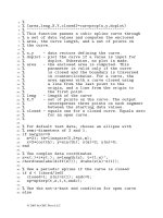
Surface Plot of a General Polyhedron
y axis
z axis
Figure 5.6: Surface Plot of a General Polyhedron
© 2003 by CRC Press LLC
GAUSS INTEGRATION WITH GEOMETRIC PROPERTY APPLICATIONS 185
Program polhdrun
1: function polhdrun
2: % Example: polhdrun
3: % ~~~~~~~~~~~~~~~~~

4: %
5: % This program illustrates the use of routine
6: % polhedrn to calculate the geometrical
7: % properties of a polyhedron.
8: %
9: % User m functions called:
10: % crosmat, polyxy, cubrange, pyramid,
11: % polhdplt, polhedrn
12:
13:
x=[2 2 2 2 2 2 0 0 0 0 0 0]-1;
14: y=[0 4 4 2 3 3 0 4 4 2 3 3];
15: z=[0 0 4 1 1 2 0 0 4 1 1 2];
16: idface=[1 2 365463;
17: 13970000;
18: 17820000;
19: 28930000;
20: 7 9 12 10 11 12 9 8;
21: 4101260000;
22: 4511100000;
23: 5612110000];
24: polhdplt(x,y,z,idface,[1,1,1]);
25: [v,rc,vrr,irr]=polhedrn(x,y,z,idface)
26:
27:
%=============================================
28:
29:
function [v,rc,vrr,irr]=polhedrn(x,y,z,idface)
30: %

31: % [v,rc,vrr,irr]=polhedrn(x,y,z,idface)
32: % ~~~~~~~~~~~~~~~~~~~~~~~~~~~~~~~~~
33: %
34: % This function determines the volume,
35: % centroidal coordinates and inertial moments
36: % for an arbitrary polyhedron.
37: %
38: % x,y,z - vectors containing the corner
39: % indices of the polyhedron
40: % idface - a matrix in which row j defines the
41: % corner indices of the j’th face.
© 2003 by CRC Press LLC
186 ADVANCED MATH AND MECHANICS APPLICATIONS USING MATLAB
42: % Each face is traversed in a
43: % counterclockwise sense relative to
44: % the outward normal. The column
45: % dimension equals the largest number
46: % of indices needed to define a face.
47: % Rows requiring fewer than the
48: % maximum number of corner indices are
49: % padded with zeros on the right.
50: %
51: % v - the volume of the polyhedron
52: % rc - the centroidal radius
53: % vrr - the integral of R*R’*d(vol)
54: % irr - the inertia tensor for a rigid body
55: % of unit mass obtained from vrr as
56: % eye(3,3)*sum(diag(vrr))-vrr
57: %
58: % User m functions called: pyramid

59: %
60:
61:
r=[x(:),y(:),z(:)]; nf=size(idface,1);
62: v=0; vr=0; vrr=0;
63: for k=1:nf
64: i=idface(k,:); i=i(find(i>0));
65: [u,ur,urr]=pyramid(r(i,:));
66: v=v+u; vr=vr+ur; vrr=vrr+urr;
67: end
68: rc=vr/v; irr=eye(3,3)*sum(diag(vrr))-vrr;
69:
70:
%=============================================
71:
72:
function [area,xbar,ybar,axx,axy,ayy]=polyxy(x,y)
73: %
74: % [area,xbar,ybar,axx,axy,ayy]=polyxy(x,y)
75: % ~~~~~~~~~~~~~~~~~~~~~~~~~~~~~~~~~~~~~~~~
76: %
77: % This function computes the area, centroidal
78: % coordinates, and inertial moments of an
79: % arbitrary polygon.
80: %
81: % x,y - vectors containing the corner
82: % coordinates. The boundary is
83: % traversed in a counterclockwise
84: % direction
85: %

86: % area - the polygon area
© 2003 by CRC Press LLC
GAUSS INTEGRATION WITH GEOMETRIC PROPERTY APPLICATIONS 187
87: % xbar,ybar - the centroidal coordinates
88: % axx - integral of x^2*dxdy
89: % axy - integral of xy*dxdy
90: % ayy - integral of y^2*dxdy
91: %
92: % User m functions called: none
93: %
94:
95:
n=1:length(x); n1=n+1;
96: x=[x(:);x(1)]; y=[y(:);y(1)];
97: a=(x(n).*y(n1)-y(n).*x(n1))’;
98: area=sum(a)/2; a6=6*area;
99: xbar=a*(x(n)+x(n1))/a6; ybar=a*(y(n)+y(n1))/a6;
100: ayy=a*(y(n).^2+y(n).*y(n1)+y(n1).^2)/12;
101: axy=a*(x(n).*(2*y(n)+y(n1))+x(n1).*
102: (2*y(n1)+y(n)))/24;
103: axx=a*(x(n).^2+x(n).*x(n1)+x(n1).^2)/12;
104:
105:
%=============================================
106:
107:
function [v,vr,vrr,h,area,n]=pyramid(r)
108: %
109: % [v,vr,vrr,h,area,n]=pyramid(r)
110: % ~~~~~~~~~~~~~~~~~~~~~~~~~~~~~~

111: %
112: % This function determines geometrical
113: % properties of a pyramid with the apex at the
114: % origin and corner coordinates of the base
115: % stored in the rows of r.
116: %
117: % r - matrix containing the corner
118: % coordinates of a polygonal base stored
119: % in the rows of matrix r.
120: %
121: % v - the volume of the pyramid
122: % vr - the first moment of volume relative to
123: % the origin
124: % vrr - the second moment of volume relative
125: % to the origin
126: % h - the pyramid height
127: % area - the base area
128: % n - the outward directed unit normal to
129: % the base
130: %
131: % User m functions called: crosmat, polyxy
© 2003 by CRC Press LLC
188 ADVANCED MATH AND MECHANICS APPLICATIONS USING MATLAB
132: %
133:
134:
ns=size(r,1);
135: na=sum(crosmat(r,r([2:ns,1],:)))’/2;
136: area=norm(na); n=na/area; p=null(n’);
137: i=p(:,1); j=p(:,2);

138: if det([p,n])<0, j=-j; end;
139: r1=r(1,:); rr=r-r1(ones(ns,1),:);
140: x=rr*i; y=rr*j;
141: [areat,xc,yc,axx,axy,ayy]=polyxy(x,y);
142: rc=r1’+xc*i+yc*j; h=r1*n;
143: v=h*area/3; vr=v*3/4*rc;
144: axx=axx-area*xc^2; ayy=ayy-area*yc^2;
145: axy=axy-area*xc*yc;
146: vrr=h/5*(area*rc*rc’+axx*i*i’+ayy*j*j’+
147: axy*(i*j’+j*i’));
148:
149:
%=============================================
150:
151:
function polhdplt(x,y,z,idface,colr)
152: %
153: % polhdplt(x,y,z,idface,colr)
154: % ~~~~~~~~~~~~~~~~~~~~~~~~~~~
155: %
156: % This function makes a surface plot of an
157: % arbitrary polyhedron.
158: %
159: % x,y,z - vectors containing the corner
160: % indices of the polyhedron
161: % idface - a matrix in which row j defines the
162: % corner indices of the j’th face.
163: % Each face is traversed in a
164: % counterclockwise sense relative to
165: % the outward normal. The column

166: % dimension equals the largest number
167: % of indices needed to define a face.
168: % Rows requiring fewer than the
169: % maximum number of corner indices are
170: % padded with zeros on the right.
171: % colr - character string or a vector
172: % defining the surface color
173: %
174: % User m functions called: cubrange
175: %
176:
© 2003 by CRC Press LLC
GAUSS INTEGRATION WITH GEOMETRIC PROPERTY APPLICATIONS 189
177: if nargin<5, colr=[1 0 1]; end
178: hold off, close; nf=size(idface,1);
179: v=cubrange([x(:),y(:),z(:)],1.1);
180: for k=1:nf
181: i=idface(k,:); i=i(find(i>0));
182: xi=x(i); yi=y(i); zi=z(i);
183: fill3(xi,yi,zi,colr); hold on;
184: end
185: axis(v); grid on;
186: xlabel(’x axis’); ylabel(’y axis’);
187: zlabel(’z axis’);
188: title(’Surface Plot of a General Polyhedron’);
189: figure(gcf); hold off;
190:
191:
%=============================================
192:

193:
function c=crosmat(a,b)
194: %
195: % c=crosmat(a,b)
196: % ~~~~~~~~~~~~~~
197: %
198: % This function computes the vector cross
199: % product for vectors stored in the rows
200: % of matrices a and b, and returns the
201: % results in the rows of c.
202: %
203: % User m functions called: none
204: %
205:
206:
c=[a(:,2).*b(:,3)-a(:,3).*b(:,2),
207: a(:,3).*b(:,1)-a(:,1).*b(:,3),
208: a(:,1).*b(:,2)-a(:,2).*b(:,1)];
209:
210:
%=============================================
211:
212:
% function range=cubrange(xyz,ovrsiz)
213: % See Appendix B
© 2003 by CRC Press LLC
190 ADVANCED MATH AND MECHANICS APPLICATIONS USING MATLAB
5.8 Evaluating Integrals Having Square Root Type Singularities
Consider the problem of evaluating the following three integrals having square
root type singularities at one or both ends of the integration interval:

I
1
=
b

a
f(x)
√
x − a
dx , I
2
=
b

a
f(x)
√
b − x
dx , I
3
=
b

a
f(x)

(x − a)(b − x)
dx.
The singularities in these integrals can be removed using substitutions x − a =
t

2
,b− x = t
2
, and (x −a)(b − x)=(b + a)/2+(b − a)/2cos(t) which lead to
I
1
=2
√
b−a

0
f(a + t
2
) dt , I
2
=2
√
b−a

0
f(b − t
2
) dt
I
3
=
π

0
f(

b + a
2
+
b − a
2
cos(t))dt.
These modiÞed integrals can be evaluated using gcquad or quadl by creating in-
tegrands with appropriate argument shifts. Two integration functions quadgsqrt
and quadlsqrt were written to handle each of the three integral types. Shown be-
low is a program called sqrtquadtest which computes results for the case where
f(x)=e
ux
cos(vx) with constants u and v being parameters passed to the inte-
grators using the varargin construct in MATLAB. Function quadgsqrt uses Gauss
quadrature to evaluate I
1
and I
2
, and uses Chebyshev quadrature [1] to evaluate I
3
.
When f(x) is a polynomial, then taking parameter norder in function quadgsqrt
equal to the polynomial order gives exact results. With norder taken sufÞciently
high, more complicated functions can also be integrated accurately. Function quadl-
sqrt evaluates the three integral types using the adaptive integrator quadl, which
accommodates f(x) of quite general form. The program shown below integrates the
test function for parameter choices corresponding to [a, b, u, v]=[1, 4, 3, 10] with
norder=10 in quadgsqrt and tol=1e-12 in quadlsqrt . Output from the program
for this data case appears as comments at lines 14 thru 35 of sqrtquadtest. The
integrators apparently work well and give results agreeing to Þfteen digits. How-

ever, quadlsqrt took more than four hundred times as long to run as quadgsqrt.
Furthermore, the structure of quadgsqrt is such that it could easily be modiÞed to
accommodate a form of f(x) which returns a vector.
5.8.1 Program Listing
Singular Integral Program
1: function [vg,tg,vL,tL,pctdiff]=sqrtquadtest
© 2003 by CRC Press LLC
GAUSS INTEGRATION WITH GEOMETRIC PROPERTY APPLICATIONS 191
2: %
3: % [vg,tg,vL,tL,pctdiff]=sqrtquadtest
4: %~~~~~~~~~~~~~~~~~~~~~~~~~~~~~~~~~~~
5: % This function compares the accuracy and
6: % computation time for functions quadgsqrt
7: % and quadlsqrt to evaluate:
8: % integral(exp(u*x)*cos(v*x)/radical(x), a<x<b)
9: % where radical(x) is sqrt(x-a), sqrt(b-x), or
10: % sqrt((x-a)*(b-x))
11:
12:
%
13: % Program Output
14:
15:
% >> sqrtquadtest;
16:
17:
% EVALUATING INTEGRALS WITH SQUARE ROOT TYPE
18: % SINGULARITIES AT THE END POINTS
19:
20:

% Function integrated:
21: % ftest(x,u,v)=exp(u*x).*cos(v*x)
22:
23:
%a=1 b=4
24: %u=3 v=10
25:
26:
% Results from function gquadsqrt
27: % 4.836504484e+003 -8.060993912e+003 -4.264510048e+003
28: % Computation time = 0.0159 sec.
29:
30:
% Results from function quadlsqrt
31: % 4.836504484e+003 -8.060993912e+003 -4.264510048e+003
32: % Computation time = 7.03 sec.
33:
34:
% Percent difference for the two methods
35: % -3.6669e-012 -1.5344e-012 1.4929e-012
36: %>>
37:
38:
%
39:
40:
% The test function
41: ftest=inline(’exp(u*x).*cos(v*x)’,’x’,’u’,’v’);
42:
43:

% Limits and function parameters
44: a=1; b=4; u=3; v=10;
45:
46:
nloop=100; tic;
© 2003 by CRC Press LLC
192 ADVANCED MATH AND MECHANICS APPLICATIONS USING MATLAB
47: for j=1:nloop
48: v1g=quadgsqrt(ftest,1,a,b,40,1,u,v);
49: v2g=quadgsqrt(ftest,2,a,b,40,1,u,v);
50: v3g=quadgsqrt(ftest,3,a,b,40,1,u,v);
51: end
52: vg=[v1g,v2g,v3g]; tg=toc/nloop;
53: disp(’ ’)
54: disp(’EVALUATING INTEGRALS WITH SQUARE ROOT TYPE’)
55: disp(’ SINGULARITIES AT THE END POINTS’)
56: disp(’ ’)
57: disp(’Function integrated:’)
58: disp(’ftest(x,u,v)=exp(u*x).*cos(v*x)’)
59: disp(’ ’)
60: disp([’a = ’,num2str(a),’ b = ’,num2str(b)])
61: disp([’u = ’,num2str(u),’ v = ’,num2str(v)])
62: disp(’ ’)
63: disp(’Results from function gquadsqrt’)
64: fprintf(’%17.9e %17.9e %17.9e\n’,vg)
65: disp([’Computation time = ’,num2str(tg),’ sec.’])
66:
67:
tol=1e-12; tic;
68: v1L=quadlsqrt(ftest,1,a,b,tol,[],u,v);

69: v2L=quadlsqrt(ftest,2,a,b,tol,[],u,v);
70: v3L=quadlsqrt(ftest,3,a,b,tol,[],u,v);
71: vL=[v1L,v2L,v3L]; tL=toc;
72:
73:
disp(’ ’)
74: disp(’Results from function quadlsqrt’)
75: fprintf(’%17.9e %17.9e %17.9e\n’,vL)
76: disp([’Computation time = ’,num2str(tL),’ sec.’])
77:
78:
pctdiff=100*(vg-vL)./vL; disp(’ ’)
79: disp(’Percent difference for the two methods’)
80: fprintf(’%13.4e %12.4e %12.4e\n’,pctdiff)
81:
82:
%=========================================
83:
84:
function v=quadgsqrt(
85: func,type,a,b,norder,nsegs,varargin)
86: %
87: % v=quadgsqrt(func,type,a,b,norder,nsegs,varargin)
88: %
89: %~~~~~~~~~~~~~~~~~~~~~~~~~~~~~~~~~~~~~~~~
90: %
91: % This function evaluates an integral having a
© 2003 by CRC Press LLC
GAUSS INTEGRATION WITH GEOMETRIC PROPERTY APPLICATIONS 193
92: % square root type singularity at one or both ends

93: % of the integration interval a<x<b. Composite
94: % Gauss integration is used with func(x) treated
95: % as a polynomial of degree norder.
96: % The integrand has the form:
97: % func(x)/sqrt(x-a) if type==1.
98: % func(x)/sqrt(b-x) if type==2.
99: % func(x)/sqrt((x-a)*(b-x)) if type==3.
100: % The integration interval is subdivided into
101: % nsegs subintervals of equal length.
102: %
103: % func - a character string or function handle
104: % naming a function continuous in the
105: % interval from x=a to x=b
106: % type - 1 if the integrand is singular at x=a
107: % 2 if the integrand is singular at x=b
108: % 3 if the integrand is singular at both
109: % x=a and x=b.
110: % a,b - integration limits with b>a
111: % norder - polynomial interpolation order within
112: % each interval. Lowest norder is 20.
113: % nsegs - number of integration subintervals
114: %
115: % User m functions called: gcquad
116: %
117: % Reference: Abromowitz and Stegun, ’Handbook of
118: % Mathematical Functions’, Chapter 25
119: %
120:
121:
if nargin<6, nsegs=1; end;

122: if nargin<5, norder=50; end
123: switch type
124: case 1 % Singularity at the left end.
125: % Use Gauss quadrature
126: [dumy,bp,wf]=gcquad(
127: ’’,0,sqrt(b-a),norder+1,nsegs);
128: t=a+bp.^2; y=feval(func,t,varargin{:});
129: v=wf(:)’*y(:)*2;
130: case 2 % Singularity at the right end.
131: % Use Gauss quadrature
132: [dumy,bp,wf]=gcquad(
133: ’’,0,sqrt(b-a),norder+1,nsegs);
134: t=b-bp.^2; y=feval(func,t,varargin{:});
135: v=wf(:)’*y(:)*2;
136: case 3 % Singularity at both ends.
© 2003 by CRC Press LLC
194 ADVANCED MATH AND MECHANICS APPLICATIONS USING MATLAB
137: % Use Chebyshev integration
138: n=norder; bp=cos(pi/(2*n+2)*(1:2:2*n+1));
139: c1=(b+a)/2; c2=(b-a)/2; t=c1+c2*bp;
140: y=feval(func,t,varargin{:});
141: v=pi/(n+1)*sum(y);
142: end
143:
144:
%=========================================
145:
146:
function v=quadlsqrt(fname,type,a,b,tol,trace,varargin)
147: %

148: % v=quadlsqrt(fname,type,a,b,tol,trace,varargin)
149: % ~~~~~~~~~~~~~~~~~~~~~~~~~~~~~~~~~~~~~~~~~~~~~
150: %
151: % This function uses the MATLAB integrator quadl
152: % to evaluate integrals having square root type
153: % singularities at one or both ends of the
154: % integration interval a < x < b.
155: % The integrand has the form:
156: % func(x)/sqrt(x-a) if type==1.
157: % func(x)/sqrt(b-x) if type==2.
158: % func(x)/sqrt((x-a)*(b-x)) if type==3.
159: %
160: % func - the handle for a function continuous
161: % from x=a to x=b
162: % type - 1 if the integrand is singular at x=a
163: % 2 if the integrand is singular at x=b
164: % 3 if the integrand is singular at both
165: % x=a and x=b.
166: % a,b - integration limits with b > a
167:
168:
if nargin<6 | isempty(trace), trace=0; end
169: if nargin<5 | isempty(tol), tol=1e-8; end
170: if nargin<7
171: varargin{1}=type; varargin{2}=[a,b];
172: varargin{3}=fname;
173: else
174: n=length(varargin); c=[a,b]; varargin{n+1}=type;
175: varargin{n+2}=c; varargin{n+3}=fname;
176: end

177:
178:
if type==1 | type==2
179: v=2*quadl(@fshift,0,sqrt(b-a),
180: tol,trace,varargin{:});
181: else
© 2003 by CRC Press LLC
GAUSS INTEGRATION WITH GEOMETRIC PROPERTY APPLICATIONS 195
182: v=quadl(@fshift,0,pi,tol,trace,varargin{:});
183: end
184:
185:
%=========================================
186:
187:
function u=fshift(x,varargin)
188: % u=fshift(x,varargin)
189: % This function shifts arguments to produce
190: % a nonsingular integrand called by quadl
191: N=length(varargin); fname=varargin{N};
192: c=varargin{N-1}; type=varargin{N-2};
193: a=c(1); b=c(2); c1=(b+a)/2; c2=(b-a)/2;
194:
195:
switch type
196: case 1, t=a+x.^2; case 2, t=b-x.^2;
197: case 3, t=c1+c2*cos(x);
198: end
199:
200:

if N>3, u=feval(fname,t,varargin{1:N-3});
201: else, u=feval(fname,t); end
202:
203:
%=========================================
204:
205:
% function [val,bp,wf]=gcquad(func,xlow,
206: % xhigh,nquad,mparts,varargin)
207: % See Appendix B
5.9 Gauss Integration of a Multiple Integral
Gauss integration can be used to evaluate multiple integrals having variable limits.
Consider the instance typiÞed by the following triple integral
I =

c
2
c
1

b
2
(z)
b
1
(z)

a
2
(y,z)

a
1
(y,z)
F (x, y, z) dx dy dz.
This integral can be changed into one with constant limits by the substitutions
z = c
p
+ c
m
u, −1 ≤ u ≤ 1,
y = b
p
+ b
m
t, −1 ≤ t ≤ 1,
x = a
p
+ a
m
s, −1 ≤ s ≤ 1
© 2003 by CRC Press LLC
196 ADVANCED MATH AND MECHANICS APPLICATIONS USING MATLAB
where
c
p
=
c
2
+ c
1

2
,c
m
=
c
2
− c
1
2
,
b
p
=
b
2
+ b
1
2
,b
m
=
b
2
− b
1
2
,
a
p
=

a
2
+ a
1
2
,a
m
=
a
2
− a
1
2
.
The above integral becomes
I =

1
−1

1
−1

1
−1
c
m
b
m
a

m
f(s, t, u) ds dt du
where
f(s, t, u)=F (a
p
+ a
m
s, b
p
+ b
m
t, c
p
+ c
m
u),
a
m
= a
m
(y,z)=a
m
(b
p
+ b
m
t, c
p
+ c
m

u),
b
m
= b
m
(z)=b
m
(c
p
+ c
m
u).
Thus, the integral has the form
I =

1
−1

1
−1

1
−1
G(s, t, u) ds dt du
where
G = c
m
b
m
a

m
f.
Performing the integration over each limit using an n-point quadrature formula with
weight factors w
ı
and base points x
ı
yields
I =
n

k=1
n

=1
n

ı=1
w
k
w

w
ı
G(x
ı
,x

,x
k

).
A function allowing an integrand and integration limits of general form was devel-
oped. An example is considered where the inertial moment of a sphere having unit
radius, unit mass density, and centered at (0, 0, 0) is to be obtained about an axis
through x =2,y =0, parallel to the z-axis. The related integral
I =

1
−1

√
1−z
2
−
√
1−z
2

√
1−y
2
−z
2
−
√
1−y
2
−z
2


(x − 2)
2
+ y
2

dx dy dz
has a value of 88π/15. Shown below is a function quadit3d and related limit and
integrand functions. The function triplint(n) computes the ratio of the numerically
integrated function to the exact result. The function speciÞcation triplint(20) yields
a value of 1.000067. Even though the triple integration procedure is not computa-
tionally very fast, it is nevertheless robust enough to produce accurate results when
a sufÞciently high integration order is chosen.
© 2003 by CRC Press LLC
GAUSS INTEGRATION WITH GEOMETRIC PROPERTY APPLICATIONS 197
5.9.1 Example: Evaluating a Multiple Integral
Triple Integration Program
1: function val=triplint(n)
2: %
3: % val=triplint(n)
4: % ~~~~~~~~~~~~~~~
5: % Triple integration example on inertial
6: % moment of a sphere.
7: %
8: % User m functions called: fsphere, bs1, bs2,
9: % as1, as2
10:
11:
if nargin==0, n=20; end
12: val=quadit3d(’fsphere’,[-1,1],’bs1’,’bs2’,
13: ’as1’,’as2’,n)/(88*pi/15);

14:
15:
%=============================================
16:
17:
function s = quadit3d(f,c,b1,b2,a1,a2,w)
18: %
19: % s = quadit3d(f,c,b1,b2,a1,a2,w)
20: % ~~~~~~~~~~~~~~~~~~~~~~~~~~~~~~~
21: % This function computes the iterated integral
22: %
23: % s = integral(
24: % f(x,y,z), x=a1 a2, y=b1 b2, z=c1 c2)
25: %
26: % where a1 and a2 are functions of y and z, b1
27: % and b2 are functions of z, and c is a vector
28: % containing constant limits on the z variable.
29: % Hence, as many as five external functions may
30: % be involved in the call list. For example,
31: % when the integrand and limits are:
32: %
33: % f = x.^2+y^2+z^2
34: % a2 = sqrt(4-y^2-z^2)
35: % a1 = -a2
36: % b2 = sqrt(4-z^2)
37: % b1 = -b2
38: % c = [-2,2]
39: %
40: % Then the exact value is 128*pi/5.
© 2003 by CRC Press LLC

198 ADVANCED MATH AND MECHANICS APPLICATIONS USING MATLAB
41: % The approximation produced from a 20 point
42: % Gauss formula is accurate within .007 percent.
43: %
44: % f - a function f(x,y,z) which must return
45: % a vector value when x is a vector,
46: % and y and z are scalar.
47: % a1,a2 - integration limits on the x variable
48: % which may specify names of functions
49: % or have constant values. If a1 is a
50: % function it should have a call list
51: % of the form a1(y,z). A similar form
52: % applies to a2.
53: % b1,b2 - integration limits on the y variable
54: % which may specify functions of z or
55: % have constant values.
56: % c - a vector defined by c=[c1,c2] where
57: % c1 and c2 are fixed integration
58: % limits for the z direction.
59: % w - this argument defines the quadrature
60: % formula used. It has the following
61: % three possible forms. If w is omitted,
62: % a Gauss formula of order 12 is used.
63: % If w is a positive integer n, a Gauss
64: % formula of order n is used. If w is an
65: % n by 2 matrix, w(:,1) contains the base
66: % points and w(:,2) contains the weight
67: % factors for a quadrature formula over
68: % limits -1 to 1.
69: %

70: % s - the numerically evaluated integral
71: %
72: % User m functions called: gcquad
73: %
74:
75:
if nargin<7
76: % function gcquad generates base points
77: % and weight factors
78: n=12; [dummy,x,W]=gcquad(’’,-1,1,n,1);
79: elseif size(w,1)==1 & size(w,2)==1
80: n=w; [dummy,x,W]=gcquad(’’,-1,1,n,1);
81: else
82: n=size(w,1); x=w(:,1); W=w(:,2);
83: end
84: s=0; cp=(c(1)+c(2))/2; cm=(c(2)-c(1))/2;
85:
© 2003 by CRC Press LLC
GAUSS INTEGRATION WITH GEOMETRIC PROPERTY APPLICATIONS 199
86: for k=1:n
87: zk=cp+cm*x(k);
88: if ischar(b1), B1=feval(b1,zk);
89: else, B1=b1; end
90:
91:
if ischar(b2), B2=feval(b2,zk);
92: else, B2=b2; end
93:
94:
Bp=(B2+B1)/2; Bm=(B2-B1)/2; sj=0;

95:
96:
for j=1:n
97: yj=Bp+Bm*x(j);
98: if ischar(a1), A1=feval(a1,yj,zk);
99: else, A1=a1; end
100:
101:
if ischar(a2), A2=feval(a2,yj,zk);
102: else, A2=a2; end
103:
104:
Ap=(A2+A1)/2; Am=(A2-A1)/2;
105: fval=feval(f, Ap+Am*x, yj, zk);
106: si=fval(:).’*W(:); sj=sj+W(j)*Am*si;
107: end
108: s=s+W(k)*Bm*sj;
109: end
110: s=cm*s;
111:
112:
%=============================================
113:
114:
function v=fsphere(x,y,z)
115: %
116: % v=fsphere(x,y,z)
117: % ~~~~~~~~~~~~~~~~
118: % Integrand.
119: %

120:
121:
v=(x-2).^2+y.^2;
122:
123:
%=============================================
124:
125:
function x=as1(y,z)
126: %
127: % x=as1(y,z)
128: % ~~~~~~~~~~
129: % Lower x integration limit.
130: %
© 2003 by CRC Press LLC
200 ADVANCED MATH AND MECHANICS APPLICATIONS USING MATLAB
131:
132:
x=-sqrt(1-y.^2-z.^2);
133:
134:
%=============================================
135:
136:
function x=as2(y,z)
137: %
138: % x=as2(y,z)
139: % ~~~~~~~~~~
140: % Upper x integration limit.
141: %

142:
143:
x=sqrt(1-y.^2-z.^2);
144:
145:
%=============================================
146:
147:
function y=bs1(z)
148: %
149: % y=bs1(z)
150: % ~~~~~~~~
151: % Lower y integration limit.
152: %
153:
154:
y=-sqrt(1-z.^2);
155:
156:
%=============================================
157:
158:
function y=bs2(z)
159: %
160: % y=bs2(z)
161: % ~~~~~~~~~~
162: % Upper y integration limit.
163: %
164:
165:

y=sqrt(1-z.^2);
166:
167:
%=============================================
168:
169:
% function [val,bp,wf]=gcquad(func,xlow,
170: % xhigh,nquad,mparts,varargin)
171: % See Appendix B
© 2003 by CRC Press LLC
Chapter 6
Fourier Series and the Fast Fourier
Transform
6.1 DeÞnitions and Computation of Fourier CoefÞcients
Trigonometric series are useful to represent periodic functions. A function deÞned
for −∞ <x<∞has a period of 2π if f(x+2π)=f(x) for all x. In most practical
situations, such a function can be expressed as a complex Fourier series
f(x)=
∞

=−∞
c

e
ıx
where ı =
√
−1.
The numbers c


, called complex Fourier coefÞcients, are computed by integration as
c

=
1
2π

2π
0
f(x)e
−ıx
dx.
The Fourier series can also be rewritten using sines and cosines as
f(x)=c
0
+
∞

=1
(c

+ c
−
)cos(x)+ı(c

− c
−
)sin(x).
Denoting
a


= c

+ c
−
and b

= ı(c

− c
−
)
yields
f(x)=
1
2
a
0
+
∞

=1
a

cos(x)+b

sin(x)
which is called a Fourier sine-cosine expansion. This series is especially appealing
when f(x) is real valued. For that case c
−

= c

for all , which implies that c
0
must
be real and
a

=2 real(c

) ,b

= −2 imag(c

) for >0.
Suppose we want a Fourier series expansion for a more general function f(x)
having period p instead of 2π. If we introduce a new function g(x) deÞned by
g(x)=f

px
2π


© 2003 by CRC Press LLC
then g(x) has a period of 2π. Consequently, g(x) can be represented as
g(x)=
∞

=−∞
c


e
ıx
.
From the fact that f(x)=g(2πx/p) we deduce that
f(x)=
∞

=−∞
c

e
2πıx/p
.
A need sometimes occurs to expand a function as a series of sine terms only, or as a
series of cosine terms only. If the function is originally deÞned for 0 <x<
p
2
, then
making f(x)=−f(p − x) for
p
2
<x<pgives a series involving only sine terms.
Similarly, if f(x)=+f(p −x) for
p
2
<x<p, only cosine terms arise. Thus we get
f(x)=c
0
+

∞

=1
(c

+ c
−
)cos(2πx/p) if f(x)=f(p − x),
or
f(x)=
∞

=1
ı(c

− c
−
)sin(2πx/p) if f(x)=−f(p − x).
When the Fourier series of a function is approximated using a Þnite number of terms,
the resulting approximating function may oscillate in regions where the actual func-
tion is discontinuous or changes rapidly. This undesirable behavior can be reduced
by using a smoothing procedure described by Lanczos [60]. Use is made of Fourier
series of a closely related function
ˆ
f(x) deÞned by a local averaging process accord-
ing to
ˆ
f(x)=
1
∆


x+
∆
2
x−
∆
2
f(ζ)dζ
where the averaging interval ∆ should be a small fraction of the period p. Hence we
write ∆=αp with α<1. The functions
ˆ
f(x) and f(x) are identical as α → 0.
Even for α>0, these functions also match exactly at any point x where f(x) varies
linearly between x −
∆
2
and x +
∆
2
. An important property of
ˆ
f(x) is that it agrees
closely with f(x) for small α but has a Fourier series which converges more rapidly
than the series for f(x). Furthermore, from its deÞnition,
ˆ
f(x)=
∞

=−∞
c


1
pα

x+
αp
2
x−
αp
2
e
2πıx/p
dx =
∞

=−∞
ˆc

e
2πıx/p
where ˆc
0
= c
0
and ˆc

= c

sin(πα)/(πα) for  =0. Evidently the Fourier coef-
Þcients of

ˆ
f(x) are easily obtainable from those of f(x). When the series for f (x)
converges slowly, using the same number of terms in the series for
ˆ
f(x) often gives
an approximation preferable to that provided by the series for f(x). This process is
called smoothing.
© 2003 by CRC Press LLC
6.1.1 Trigonometric Interpolation and the Fast Fourier Transform
Computing Fourier coefÞcients by numerical integration is very time consuming.
Consequently, we are led to investigate alternative methods employing trigonometric
polynomial interpolation through evenly spaced data. The resulting formulas are the
basis of an important algorithm called the Fast Fourier Transform (FFT) . Although
the Fourier coefÞcients obtained by interpolation are approximate, these coefÞcients
can be computed very rapidly when the number of sample points is an integer power
of 2 or a product of small primes. We will discuss next the ideas behind trigonometric
polynomial interpolation among evenly spaced data values.
Suppose we truncate the Fourier series and only use harmonics up to some order
N. We assume f(x) has period 2π so that
f(x)=
N

=−N
c

e
ıx
.
This trigonometric polynomial satisÞes f(0) = f(2π) even though the original func-
tion might actually have a Þnite discontinuity at 0 and 2π. Consequently, we may

choose to use, in place of f(0), the limit as  → 0 of [f()+f(2π − )]/2.
It is well known that the functions e
ıx
satisfy an orthogonality condition for inte-
gration over the interval 0 to 2π. They also satisfy an orthogonality condition regard-
ing summation over equally spaced data. The latter condition is useful for deriving a
discretized approximation of the integral formula for the exact Fourier coefÞcients.
Let us choose data points
x

=

π
N

, 0 ≤  ≤ (2N −1),
and write the simultaneous equations to make the trigonometric polynomial match
the original function at the equally spaced data points. To shorten the notation we let
t = e
ıπ/N
,
and write
f
k
=
N

=−N
c


t
k
.
Suppose we pick an arbitrary integer n in the range −N<n<N. Multiplying the
last equation by t
−kn
and summing from k =0to 2N −1 gives
2N−1

k=0
f
k
t
−kn
=
2N−1

k=0
t
−kn
N

=−N
c

t
k
.
Interchanging the summation order in the last equation yields
2N−1


k=0
f
k
t
−kn
=
N

=−N
c

2N−1

k=0
ζ
k
© 2003 by CRC Press LLC
where ζ = e
ı(−n)π/N
. Summing the inner geometric series gives
2N−1

k=0
ζ
k
=

1−ζ
2N

1−ζ
for ζ =1,
2N for ζ =1.
We Þnd, for all k and n in the stated range, that
ζ
2N
= e
ı2π(k−n)
=1.
Therefore we get
2N−1

k=0
f
k
t
−kn
=2Nc
n
, −N<n<N.
In the cases where n = ±N, the procedure just outlined only gives a relationship
governing c
N
+ c
−N
. Since the Þrst and last terms cannot be computed uniquely, we
customarily take N large enough to discard these last two terms and write simply
c
n
=

1
2N
2N−1

k=0
f
k
t
−kn
, −N<n<N.
This formula is the basis for fast algorithms (called FFT for Fast Fourier Transform)
to compute approximate Fourier coefÞcients. The periodicity of the terms depending
on various powers of e
ıπ/N
can be utilized to greatly reduce the number of trigono-
metric function evaluations. The case where N equals a power of 2 is especially
attractive. The mathematical development is not provided here. However, the related
theory was presented by Cooley and Tukey in 1965 [21] and has been expounded in
many textbooks [53, 96]. The result is a remarkably concise algorithm which can
be comprehended without studying the details of the mathematical derivation. For
our present interests it is important to understand how to use MATLAB’s intrinsic
function for the FFT (fft).
Suppose a periodic function is evaluated at a number of equidistant points ranging
over one period. It is preferable for computational speed that the number of sample
points should equal an integer power of two (n =2
m
). Let the function values for
argument vector
x = p/n ∗ (0 : n − 1)
be an array f denoted by

f ⇐⇒ [f
1
,f
2
, ··· ,f
n
].
The function evaluation fft(f) produces an array of complex Fourier coefÞcients
multiplied by n and arranged in a peculiar fashion. Let us illustrate this result for
n =8.If
f =[f
1
,f
2
, ··· ,f
8
]
then fft(f)/8 produces
c =[c
0
,c
1
,c
2
,c
3
,c
∗
,c
−3

,c
−2
,c
−1
].
© 2003 by CRC Press LLC
The term denoted by c
∗
actually turns out to equal c
4
+ c
−4
, so it would not be used
in subsequent calculations. We generalize this procedure for arbitrary n as follows.
Let N = n/2 − 1. In the transformed array, elements with indices of 1, ··· ,N +1
correspond to c
0
, ··· ,c
N
and elements with indices of n, n − 1,n− 2, ··· ,N +
3 correspond to c
−1
,c
−2
,c
−3
, ··· ,c
−N
. It is also useful to remember that a real
valued function has c

−n
=conj(c
n
).ToÞx our ideas about how to evaluate a
Fourier series, suppose we want to sum an approximation involving harmonics from
order zero to order (nsum −1). We are dealing with a real valued function deÞned
by func with a real argument vector x. The following code expands func and sums
the series for argument x using nsum terms.
function fouval=fftaprox(func,period,nfft,nsum,x)
fc=feval(func,period/nfft*(0:nfft-1));
fc=fft(fc)/nfft; fc(1)=fc(1)/2;
w=2*pi/period*(0:nsum-1);
fouval=2*real(exp(i*x(:)*w)*fc(:));
6.2 Some Applications
Applications of Fourier series arise in numerous practical situations such as struc-
tural dynamics, signal analysis, solution of boundary value problems, and image
processing. Three examples are given below that illustrate use of the FFT. The Þrst
example calculates Bessel functions and the second problem studies forced dynamic
response of a lumped mass system. The Þnal example presents a program for con-
structing Fourier expansions and displaying graphical results for linearly interpolated
or analytically deÞned functions.
6.2.1 Using the FFT to Compute Integer Order Bessel Functions
The FFT provides an efÞcient way to compute integer order Bessel functions
J
n
(x) which are important in various physical applications [119]. Function J
n
(x)
can be obtained as the complex Fourier coefÞcient of e
ınθ

in the generating function
described by
e
ıx sin(θ)
=
∞

n=−∞
J
n
(x)e
ınθ
.
Orthogonality conditions imply
J
n
(x)=
1
2π

2π
0
e
ı(x sin(θ)−nθ)
dθ.
© 2003 by CRC Press LLC
0
5
10
15

20
0
5
10
15
20
−0.4
−0.2
0
0.2
0.4
0.6
0.8
1
argument x
Surface Plot For J
n
(x)
order n
function value
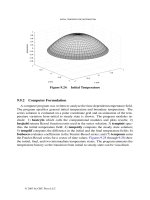
Figure 6.1: Surface Plot for J
n
(x)
The Fourier coefÞcients represented by J
n
(x) can be computed approximately with
the FFT. The inÞnite series converges very rapidly because the function it represents
has continuous derivatives of all Þnite orders. Of course, e
ıx sin(θ)
is highly oscilla-

tory for large |x|, thereby requiring a large number of sample points in the FFT to
obtain accurate results. For n<30 and |x| < 30, a 128-point transform is adequate
to give about ten digit accuracy for values of J
n
(x). The following code implements
the above ideas and plots a surface showing how J
n
changes in terms of n and x.
© 2003 by CRC Press LLC
MATLAB Example
Bessel Function Program plotjrun
1: function plotjrun
2: % Example: plotjrun
3: % ~~~~~~~~~~~~~~~~~
4: % This program computes integer order Bessel
5: % functions of the first kind by using the FFT.
6: %
7: % User m functions required: jnft
8:
9:
x=0:.5:20; n=0:20; J=jnft(n,x); surf(x,n,J’);
10: title(’Surface Plot For J_{n}(x)’);
11: ylabel(’order n’), xlabel(’argument x’)
12: zlabel(’function value’), figure(gcf);
13: print -deps plotjrun
14:
15:
%==============================================
16:
17:

function J=jnft(n,z,nft)
18: %
19: % J=jnft(n,z,nft)
20: % ~~~~~~~~~~~~~~~~~~~~~
21: % Integer order Bessel functions of the
22: % first kind computed by use of the Fast
23: % Fourier Transform (FFT).
24: %
25: % n - integer vector defining the function
26: % orders
27: % z - a vector of values defining the
28: % arguments
29: % nft - number of function evaluations used
30: % in the FFT calculation. This value
31: % should be an integer power of 2 and
32: % should exceed twice the largest
33: % component of n. When nft is omitted
34: % from the argument list, then a value
35: % equal to 512 is used. More accurate
36: % values of J are computed as nft is
37: % increased. For max(n) < 30 and
38: % max(z) < 30, nft=256 gives about
39: % ten digit accuracy.
40: % J - a matrix of values for the integer
© 2003 by CRC Press LLC
41: % order Bessel function of the first
42: % kind. Row position matches orders
43: % defined by n, and column position
44: % corresponds to arguments defined by
45: % components of z.

46: %
47: % User m functions called: none.
48: %
49:
50:
if nargin<3, nft=512; end;
51: J=exp(sin((0:nft-1)’*
52: (2*pi/nft))*(i*z(:).’))/nft;
53: J=fft(J); J=J(1+n,:).’;
54: if sum(abs(imag(z)))<max(abs(z))/1e10
55: J=real(J);
56: end
6.2.2 Dynamic Response of a Mass on an Oscillating Foundation
Fourier series are often used to describe time dependent phenomena such as earth-
quake ground motion. Understanding the effects of foundation motions on an elastic
structure is important in design. The model in Figure 6.2 embodies rudimentary as-
pects of this type of system and consists of a concentrated mass connected by a spring
and viscous damper to a base which oscillates with known displacement Y (t). The
system is assumed to have arbitrary initial conditions y(0) = y
0
and ˙y(0) = v
0
when
the base starts moving. The resulting displacement and acceleration of the mass are
to be computed.
We assume that Y (t) can be represented well over some time interval p by a Four-
ier series of the form
Y (t)=
∞


n=−∞
c
n
e
ıω
n
t
,ω
n
=
2nπ
p
where c
−n
= conj(c
n
) because Y is real valued. The differential equation governing
this problem is
m¨y + c ˙y + ky = kY (t)+c
˙
Y (t)=F (t)
where the forcing function can be expressed as
F (t)=
∞

n=−∞
c
n
[k + ıcω
n

]e
ıω
n
t
= kc
0
+2real

∞

n=1
f
n
e
ıω
n
t

and
f
n
= c
n
(k + ıcω
n
).
The corresponding steady-state solution of the differential equation is representable
© 2003 by CRC Press LLC