Aerodynamics for engineering students - part 5 pot
Bạn đang xem bản rút gọn của tài liệu. Xem và tải ngay bản đầy đủ của tài liệu tại đây (1.82 MB, 67 trang )
230
Aerodynamics
for
Engineering
Students
Fig.
5.20
Modelling the displacement effect by a distribution
of
sources
wings having high aspect ratio, intuition would suggest that the flow over most
of
the
wing behaves as if it were two-dimensional. Plainly this will not be a good approxi-
mation near the wing-tips where the formation of the trailing vortices leads to highly
three-dunensional flow. However, away from the wing-tip region, Eqn (5.23) reduces
approximately to Eqn (4.103) and, to a good approximation, the
C,
distributions
obtained for symmetrical aerofoils can be used for the wing sections. For complete-
ness
this
result is demonstrated formally immediately below. However, if this is not of
interest go directly to the next section.
Change the variables in Eqn (5.23) to
%
=
(x
-
xI)/c,
21
=
z1/c and
Z
=
(z
-
z1)/c.
Now provided that the non-dimensional shape of the wing-section does not change
along the span, or, at any rate, only changes very slowly
St
=
d(yt/c)/dZ does not
vary with
Z
and the integral
I1
in Eqn (5.23) becomes
"
12
To
evaluate the integral
12
change variable to
x
=
l/Z
so
that
1
11
1
1
Finite
wing
theory
231
For large aspect ratios
s
>>
cy
so
provided
z1
is not close to
fs,
i.e. near the wing-tips,
giving
Thus Eqn (5.23) reduces to the two-dimensional result, Eqn (4.103), i.e.
(5.24)
Lifting effect
To
understand the fundamental concepts involved in modelling the lifting effect of
a vortex sheet, consider first the simple rectangular wing depicted in Fig. 5.21. Here
the vortex sheet is constructed from a collection of horseshoe vortices located in the
y
=
0
plane.
From Helmholtz's second theorem (Section 5.2.1) the strength of the circulation
round any section of the vortex sheet (or wing) is the
sum
of the strengths of the
vortex
filaments
CL\
Fig.
5.21
The
relation between spanwise load variation and trailing vortex strength
232
Aerodynamics
for
Engineering Students
vortex filaments cut by the section plane.
As
the section plane is progressively moved
outwards from the centre section to the tips, fewer and fewer bound vortex filaments
are left for successive sections to cut
so
that the circulation around the sections
diminishes.
In
this way, the spanwise change in circulation round the wing is related
to the spanwise lengths of the bound vortices. Now, as the section plane is moved
outwards along the bound bundle of filaments, and as the strength of the bundle
decreases, the strength of the vortex filaments
so
far shed must increase, as the overall
strength
of
the system cannot diminish. Thus the change in circulation from section
to section is equal to the strength of the vorticity shed between these sections.
Figure 5.21 shows a simple rectangular wing shedding a vortex trail with each pair
of
trailing vortex filaments completed by a spanwise bound vortex. It will be noticed
that a line joining the ends of all the spanwise vortices forms a curve that, assuming
each vortex is
of
equal strength and given a suitable scale, would be a curve of the
total strengths of the bound vortices at any section plotted against the span. This
curve has been plotted for clarity
on
a spanwise line through the centre of pressure of
the wing and is a plot of (chordwise) circulation
(I')
measured on a vertical ordinate,
against spanwise distance from the centre-line
(CL)
measured
on
the horizontal
ordinate. Thus at a section
z
from the centre-line sufficient hypothetical bound
vortices are cut to produce a chordwise circulation around that section equal to
I'.
At a further section
z
+
Sz
from the centre-line the circulation has fallen to
l?
-
ST,
indicating that between sections
z
and
z
+
Sz
trailing vorticity to the strength of
SI'
has been shed.
If the circulation curve can be described as some function of
z,flz)
say then the
strength of circulation shed
(5.25)
Now at any section the lift per span is given by the Kutta-Zhukovsky theorem
Eqn
(4.10)
I=pVT
and for a given flight speed and air density,
I'
is thus proportional to
1.
But
I
is the
local intensity of lift or lift grading, which is either known or is the required quantity
in the analysis.
The substitution of the wing by a system of bound vortices has not been rigorously
justified at
this
stage. The idea allows a relation to be built up between the physical
load distribution
on
the wing, which depends,
as
shall be shown, on the wing
geometric and aerodynamic parameters, and the trailing vortex system.
(a)
It
will be noticed from the leading sketch that the trailing filaments are closer
together when they are shed from a rapidly diminishing or changing distribution
curve. Where the filaments are closer the strength of the vorticity is greater. Near
the tips, therefore, the shed vorticity is the most strong, and at the centre where
the distribution curve is flattened out the shed vorticity is weak to infinitesimal.
(b)
A
wing infinitely long in the spanwise direction, or in two-dimensional flow, will
have constant spanwise loading. The bundle will have filaments all of equal
length and none will be turned back to
form
trailing vortices. Thus there is
no
trailing vorticity associated with two-dimensional wings. This is capable of
deduction by a more direct process, i.e. as the wing is infinitely long in the
spanwise direction the lower surface @ugh) and upper surface (low) pressures
Figure 5.21 illustrates two further points:
Finite wing theory
233
cannot tend to equalize by spanwise components of velocity
so
that the streams
of air meeting at the trailing edge after sweeping under and over the wing have no
opposite spanwise motions but join up in symmetrical flow in the direction of
motion. Again no trailing vorticity is formed.
A
more rigorous treatment of the vortex-sheet modelling is now considered. In
Section 4.3 it was shown that, without loss of accuracy, for thin aerofoils the vortices
could be considered as being distributed along the chord-line, i.e. the
x
axis, rather
than the camber line. Similarly, in the present case, the vortex sheet can be located on
the
(x,
z)
plane, rather than occupying the cambered and possibly twisted mid-surface
of
the wing. This procedure greatly simplifies the details of the theoretical modelling.
One of the infinitely many ways of constructing a suitable vortex-sheet model is
suggested by Fig. 5.21.
This
method is certainly suitable for wings with a simple
planform shape, e.g. a rectangular wing. Some wing shapes for which it is not at all
suitable are shown in Fig. 5.22. Thus for the general case an alternative model is
required. In general, it is preferable to assign an individual horseshoe vortex of
strength
k
(x,
z)
per unit chord
to
each element of wing surface (Fig. 5.23). This
method of constructing the vortex sheet leads
to
certain mathematical difficulties
(a
1
Delta
wing
(
b
)
Swept
-
back
wing
Fig.
5.22
Fig.
5.23
Modelling
the
lifting effect by
a
distribution
of
horseshoe
vortex
elements
234
Aerodynamics
for
Engineering Students
Strength,
ksxl
/,
Strength,
(kt
all
ak
6z,)8xl
,Strength,
kSx,
___
I
I
I
1
kZngth,
-
81,
sx,
1
(a
)
Horseshoe vortices
(b)
L-shaped vortices
Fig.
5.24
Equivalence between distributions
of
(a) horseshoe and (b) L-shaped vortices
when calculating the induced velocity. These problems can be overcome by recom-
bining the elements in the way depicted in Fig. 5.24. Here it is recognized that partial
cancellation occurs for two elemental horseshoe vortices occupying adjacent span-
wise positions,
z
and
z
+
6z. Accordingly, the horseshoe-vortex element can be
replaced by the L-shaped vortex element shown in Fig. 5.24. Note that although this
arrangement appears to violate Helmholtz’s second theorem, it is merely a math-
ematically convenient way of expressing the model depicted in Fig. 5.23 which fully
satisfies this theorem.
5.5
Relationship between spanwise loading
and trailing vorticity
It is shown below in Section 5.5.1 how to calculate the velocity induced by
the elements
of
the vortex sheet that notionally replace the wing. This is an essential
step in the development of a general wing theory. Initially, the general case
is considered. Then it is shown how the general case can be very considerably
simplified in the special case of wings of high aspect ratio. The general case is
then dropped, to be taken up again in Section 5.8, and the assumption of large aspect
ratio is made for Section 5.6 and the remainder of the present section. Accordingly,
some readers may wish to pass over the material immediately below and go
directly to the alternative derivation of Eqn (5.32) given at the end of the present
section.
5.5.1
Induced velocity (downwash)
Suppose that it is required to calculate the velocity induced at the point
Pl(x1,
zl)
in
the
y
=
0
plane by the L-shaped vortex element associated with the element of wing
surface located at point
P
(x,
z)
now relabelled A (Fig. 5.25).
Finite
wing
theoly
235
t=
2-11
I
A
/B
x-xj-/4q
p1
C
Fig.
5.25
Geometric
notation
for
L-shaped
vortex element
Making use of
Eqn
(5.9)
it can be seen that this induced velocity is perpendicular to
the
y
=
0
plane and can be written as
svi(xl,~~)
=
(svi),,
+
(6vi)Bc
-_
-
ksx
[cosel
-cos
(5.26)
4n(x
-
XI)
From the geometry of Fig.
5.25
the various trigonometric expressions in Eqn
(5.26)
can be written
as
z
-
z1
cOsel
=
cose2
=
-
&x
-
Xd2
+
(2
-
x
-
x1
J(x
-
+
(z
+
sz
-
z1)2
z
+
sz
-
21
COS
e2
+
-
=
-
sin02
=
(2
J(x
-
+
(2
+
sz
-
The binomial expansion, i.e.
(a
+
b)"
=
d
+
nd-lb
+
*.
.
;
can be used to expand some
of
the terms, for example
where
r
=
d(x
-XI)'
+
(z
-
~1)~.
In
this way, the trigonometric expressions given
above can be rewritten as
236
Aerodynamics
for
Engineering Students
(5.27)
(5.28)
(5.29)
Equations (5.27 to 5.29) are now substituted into Eqn (5.26), and terms involving
(6~)~
and higher powers are ignored, to give
In order to obtain the velocity induced at
P1
due to all the horseshoe vortex elements,
6vi
is integrated over the entire wing surface projected on to the
(x,
z)
plane. Thus
using Eqn (5.30) leads to
The induced velocity at the wing itself and in its wake is usually in a downwards
direction and accordingly, is often called the
downwash,
w,
so
that
w
=
-Vi.
It would be a difficult and involved process to develop wing theory based
on
Eqn (5.31) in its present general form. Nowadays, similar vortex-sheet models are
used by the panel methods, described in Section 5.8, to provide computationally
based models of the flow around a wing, or an entire aircraft. Accordingly, a
discussion of the theoretical difficulties involved in using vortex sheets to model wing
flows will be postponed to Section 5.8. The remainder of the present section and
Section 5.6 is devoted solely to the special case of unswept wings having high aspect
ratio. This is by no means unrealistically restrictive, since aerodynamic considera-
tions tend to dictate the use of wings with moderate to high aspect ratio for low-speed
applications such as gliders, light aeroplanes and commuter passenger aircraft. In
this special case Eqn (5.31) can be very considerably simplified.
This simplification is achieved as follows. For the purposes of determining the
aerodynamic characteristics of the wing it is only necessary to evaluate the induced
velocity at the wing itself. Accordingly the ranges for the variables of integration are
given by
-s
5
z
5
s
and
0
5
x
5
(c)
For
high
aspect ratios
S/C>
1
so
that
Ix
-
XI
I
<<
r
over most of the range of integration. Consequently, the contributions of
terms
(b)
and (c) to the integral
in
Eqn (5.31) are very small compared to that
of
term
(a) and can therefore be neglected. This allows Eqn (5.31) to be simplified to
where, as explained
in
Section 5.4.1
,
owing to Helmholtz's second theorem
(5.32)
(5.33)
Finite wing theoly
237
Fig.
5.26
Prandtl's
lifting
line
model
is the total circulation due to all the vortex filaments passing through the wing section
at
z.
Physically the approximate theoretical model implicit in Eqn
(5.32)
and
(5.33)
corresponds to replacing the wing by a single bound vortex having variable strength
I',
the so-called
Zijting
Zine
(Fig.
5.26).
This model, together with Eqns
(5.32)
and
(5.33),
is the basis of Prandtl's general wing theory which is described in Section
5.6.
The more involved theories based on the full version of Eqn
(5.31)
are usually
referred to as
lifting
surface
theories.
Equation
(5.32)
can also be deduced directly from the simple, less general, theor-
etical model illustrated in Fig.
5.21.
Consider now the influence of the trailing vortex
filaments of strength
ST
shed from the wing section at
z
in Fig.
5.21.
At some other
point z1 along the span, according to Eqn
(5.1
l),
an induced velocity equal to
will
be
felt in the downwards direction in the usual case of positive vortex strength.
All elements of shed vorticity along the span add their contribution to the induced
velocity at
z1
so
that the total influence of the trailing system at z1 is given by Eqn
(5.32).
5.5.2
The consequences
of
downwash
-
trailing vortex drag
The induced velocity at
z1
is, in general, in a downwards direction and is sometimes
called downwash. It has two very important consequences that modify the
flow
about the wing and alter its aerodynamic characteristics.
Firstly, the downwash that has been obtained for the particular point
z1
is felt to
a lesser extent ahead of
z1
and to a greater extent behind (see Fig.
5.27),
and has the
effect of tilting the resultant oncoming flow at the wing (or anywhere else within its
influence) through an angle
where
w
is the local downwash. This reduces the effective incidence
so
that for the
same lift as the equivalent infinite wing or two-dimensional wing at incidence
ax
an
incidence
a
=
am
+
E
is required at that section on the finite wing. This is illustrated
in Fig.
5.28,
which in addition shows how the two-dimensional lift
L,
is normal to
238
Aerodynamics
for
Engineering
Students
I
44
J.
J
ti444
tJ4J
4
J
c
J.1
w
=zero
WCP
w=2wcp
-
I
Fig. 5.27
Variation in magnitude
of
downwash in front
of
and behind wing
the resultant velocity
VR
and is, therefore, tilted back against the actual direction of
motion of the wing
V.
The two-dimensional lift
L,
is resolved into the aerodynamic
forces L and
D,
respectively, normal to and against the direction of the forward
velocity of the wing. Thus the second important consequence of downwash emerges.
This is the generation of a drag force
D,.
This is so important that the above
sequence will be explained in an alternative way.
A section of a wing generates a circulation of strength
I?.
This
circulation super-
imposed on an apparent oncoming flow velocity
V
produces a lift force
L,
=
pVF
according to the Kutta-Zhukovsky theorem
(4.10),
which is normal to the apparent
oncoming flow direction. The apparent oncoming flow felt by the wing section is the
resultant of the forward velocity and the downward induced velocity arising from the
trailing vortices.
Thus
the aerodynamic force L, produced by the combination of
I?
and
Y
appears as a lift force L normal to the forward motion and a drag force
D,
against the normal motion. This drag force is called
trailing vortex drug,
abbreviated
to
vortex drag
or more commonly
induced drug
(see Section
1.5.7).
Considering for a moment the wing as a whole moving through air at rest at
infinity, two-dimensional wing theory suggests that, taking air as being of small to
negligible viscosity, the static pressure of the free stream ahead is recovered behind
the wing. This means roughly that the kinetic energy induced in the flow is converted
back to pressure energy and zero drag results. The existence
of
a
thin boundary layer
and narrow wake is ignored but this does not really modify the argument.
In addition to this motion of the airstream, a finite wing spins the airflow near the
tips into what eventually becomes two trailing vortices of considerable core size. The
generation of these vortices requires a quantity
of
kinetic energy that is not recovered
Fig.
5.28
The influence
of
downwash on wing velocities and forces:
w
=
downwash;
V
=
forward
speed
of
wing;
V,
=
resultant oncoming flow at wing;
a
=
incidence;
E
=
downwash angle
=
w/V;
am
=
(g
E)
=
equivalent two-dimensional incidence;
L,
=
two-dimensional lift;
L
=
wing
lift;
D,
=trailing vortex drag
Finite wing
theory
239
by the wing system and that in fact is lost to the wing by being left behind. This
constant expenditure of energy appears to the wing as the induced
drag.
In what
follows, a third explanation of this important consequence of downwash will be of
use. Figure
5.29
shows the two velocity components of the apparent oncoming flow
superimposed
on
the circulation produced by the wing. The forward flow velocity
produces the lift and the downwash produces the vortex drag per unit span.
Thus the lift per unit span of a finite wing
(I)
(or the load grading) is by the Kutta-
Zhukovsky theorem:
I
=
pvr
the total lift being
L
=
/:pVTdz
(5.34)
The induced drag per unit span
(d,),
or the induced drag grading, again
by
the
Kutta-Zhukovsky theorem is
d,
=
pwr
(5.35)
and by similar integration over the span
D,
=
/:pwrdz
(5.36)
This expression for
D,
shows conclusively that if
w
is zero all along the span then
D,
is zero also. Clearly, if there is
no
trailing vorticity then there will be no induced drag.
This condition arises when a wing is working under two-dimensional conditions, or if
all sections are producing zero lift.
As
a consequence of the trailing vortex system, which is produced by the basic
lifting action of a (finite span) wing, the wing characteristics are considerably modi-
fied, almost always adversely, from those of the equivalent two-dimensional wing of
the same section. Equally, a wing with
flow
systems that more nearly approach the
two-dimensional case will have better aerodynamic characteristics than one where
I
=pvr
L=
f
spl/rdz
-S
d,
=pwr
Fig.
5.29
Circulation superimposed on forward wind velocity and downwash
to
give lift and vortex drag
(induced drag) respectively
240
Aerodynamics
for
Engineering Students
the end-effects are more dominant. It seems therefore that a wing that is large in the
spanwise dimension, i.e. large aspect ratio, is a better wing
-
nearer the ideal
-
than
a short span wing of the same section. It would thus appear that a wing of large
aspect ratio will have better aerodynamic characteristics than one of the same section
with a lower aspect ratio. For this reason, aircraft for which aerodynamic efficiency is
paramount have wings of high aspect ratio.
A
good example is the glider. Both the
man-made aircraft and those found in nature, such as the albatross, have wings with
exceptionally high aspect ratios.
In general, the induced velocity also varies in the chordwise direction, as is evident
from Eqn (5.31). In effect, the assumption of high aspect ratio, leading to Eqn (5.32),
permits the chordwise variation to be neglected. Accordingly, the lifting character-
istics of a section from a wing of high aspect ratio at a local angle of incidence
a(z)
are identical to those for a two-dimensional wing at an effective angle of incidence
a(z)
-
e.
Thus Prandtl's theory shows how the two-dimensional aerofoil character-
istics can be used to determine the lifting characteristics of wings of finite span. The
calculation of the
induced
angle
of
incidence
E
now becomes the central problem. This
poses certain difficulties because
E
depends on the circulation, which in turn is closely
related to the lift per unit span. The problem therefore, is to some degree circular in
nature which makes a simple direct approach to its solution impossible. The required
solution procedure is described in Section 5.6.
Before passing to the general theory in Section 5.6, whereby the spanwise circula-
tion distribution must be determined as part of the overall process, the much simpler
inverse problem
of
a
specified spanwise circulation distribution is considered in some
detail in the next subsection. Although this is a special case it nevertheless leads to
many results of practical interest. In particular, a simple quantitative result emerges
that reinforces the qualitative arguments given above concerning the greater aero-
dynamic efficiency of wings with high aspect ratio.
5.5.3
The
characteristics
of
a simple symmetric
loading
-
elliptic distribution
In
order
to
demonstrate the general method of obtaining the aerodynamic charac-
teristics of a wing from its loading distribution the simplest load expression for
symmetric flight is taken, that is a semi-ellipse. In addition, it will be found to be a
good approximation to many (mathematically) more complicated distributions and
is thus suitable for use as first predictions in performance estimates.
The spanwise variation in circulation is taken to be represented by a semi-ellipse
having the span
(2s)
as major
axis
and the circulation at mid-span
(ro)
as the semi-
minor
axis
(Fig. 5.30). From the general expression for an ellipse
or
(5.37)
This
expression can now be substituted in Eqns (5.32),
(5.34)
and (5.36) to find the
lift, downwash and vortex drag on the wing.
Finite
wing
theory
241
Fig.
5.30
Elliptic
loading
Lift
for elliptic distribution
From
Eqn
(5.34)
i.e.
whence
S
L
=
pvTo7r-
2
or introducing
1
2
L
=
CL-pvZs
(5.38)
(5.39)
giving the mid-span circulation in terms of the overall aerofoil lift coefficient and
geometry.
Downwash
for elliptic distribution
Here
Substituting this in
Eqn
(5.32)
wz,
=
z
dz
dG(Z
-
z1)
242
Aerodynamics
for
Engineering Students
Writing the numerator as
(z
-
zl)
+
z1:
1
=$[I
sdz
+zl
Js
dz
47rs
-s&E-7
-sd?Zf(z-z1)
Evaluating the first integral which is standard and writing
I
for the second
(5.40)
Now as this is a symmetric flight case, the shed vorticity is the same from each side of
the wing and the value of the downwash at some point
z1
is identical to that at the
corresponding point
-
z1 on the other wing.
TO
47rs
wz,
=-[7r+z1l]
So
substituting for fzl in Eqn
(5.40)
and equating:
This
identity is satisfied only if
I
=
0,
so
that for any point
z
-
z1 along the span
r0
4s
w=-
This
important result shows that the downwash is constant along the span.
Induced drag (vortex drag) for elliptic distribution
From Eqn
(5.36)
whence
A2
8
D~
=
-pro
Introducing
1
2
e,
vs
Dv
=
Co,-pV2S
and from Eqn
(5.39)
ro
=-
TS
Eqn
(5.42)
gives
1
CLVS
eo,
-
2
P
v2s
=
5
P
( F)
(5.41)
(5.42)
or
(5.43)
Finite
wing
theory
243
since
4s2 span2
S
area
-
aspect ratio(AR)
-
Equation (5.43) establishes quantitatively how
CDv
falls with a rise in
(AR)
and
confirms the previous conjecture given above, Eqn (5.36), that at zero lift in
sym-
metric flight
CD,
is zero and the other condition that as
(AR)
increases (to infinity for
two-dimensional flow)
CD,
decreases (to zero).
5.5.4
The general (series) distribution
of
lift
In the previous section attention was directed to distributions of circulation (or lift) along
the span in which the load is assumed to fall symmetrically about the centre-line according
to a particular family of load distributions. For steady symmetric manoeuvres this is quite
satisfactory and the previous distribution formula may
be
arranged to suit certain cases.
Its use, however, is strictly limited and it is necessary to
seek
further for an expression that
will satisfy every possible combination
of
wing design parameter and flight manoeuvre.
For example, it has so far been assumed that the wing was an isolated lifting surface that
in straight steady flight had a load distribution rising steadily from zero at the tips to a
maximum at mid-span (Fig. 5.31a). The general wing, however,
will
have a fuselage
located
in
the centre sections that will modify the loading in that region (Fig. 5.31b), and
engine nacelles or other excrescences may deform the remainder of the curve locally.
The load distributions on both the isolated wing and the general aeroplane wing will
be considerably changed in anti-symmetric flight. In rolling, for instance, the upgoing
wing suffers a large decrease in lift, which may become negative at some incidences
(Fig. 5.3 IC). With ailerons in operation the curve of spanwise loading for a wing
is
no
longer smooth and symmetrical but can be rugged and distorted in shape (Fig. 5.31d).
It is clearly necessary to find an expression that will accommodate all these various
possibilities. From previous work the formula
1
=
p
VI'
for any section of span is familiar.
Writing
I
in the
form
of the non-dimensional lift coefficient and equating to
pVT:
CL
r=-vc
2
(5.44)
is easily obtained. This shows that for a given steady flight state the circulation at any
section can be represented by the product of the forward velocity and the local chord.
Isolated wing in
flight
(am steady symmetric
I
I
I
I
(b)
I
Lift distribution
modified
by
fuselage effects
I
I
I
I
(dm
Antisymmetric flight
with ailerons
in operation
Fig.
5.31
Typical
spanwise distributions
of
lift
244
Aerodynamics
for
Engineering
Students
Now in addition the local chord
can
be expressed as a fraction of the semi-span
s,
and
with this fraction absorbed in a new number and the numeral
4
introduced for later
convenience,
I?
becomes:
r
=
4crs
where
Cr
is dimensionless circulation which will vary similarly to
r
across
the span.
In
other words,
Cr
is the shape parameter or variation of the
I'
curve and being
dimensionless it can be expressed as the Fourier sine series
ETA,
sin
ne
in which the
coefficients
A,,
represent the amplitudes, and the
sum
of the successive harmonics
describes the shape. The sine series was chosen to satisfy the end conditions of the
curve
reducing to zero at the tips where
y
=
As.
These correspond to the values of
0
=
0
and
R.
It is well understood that such a series is unlimited in angular measure
but the portions beyond
0
and
n
can be disregarded here. Further, the series can fit
any shape of curve but, in general, for rapidly changing distributions as shown by
a
rugged curve, for example, many harmonics are required to produce a sum that is
a good representation.
In
particular the series is simplified for the symmetrical loading case when the even
terms disappear (Fig.
5.32
01)). For the symmetrical case a maximum or minimum
must appear at the mid-section. This is only possible for sines of odd values of
742
That is, the symmetrical loading must be the
sum
of symmetrical harmonics. Odd
I
x
7r
2
0
-S
0
S
Fig.
5.32
Loading make-up
by
selected
sine series
Finite
wing
theory
245
harmonics are symmetrical. Even harmonics,
on
the other hand, return to zero again
at
7r/2
where in addition there is always a change in sign. For any asymmetry in the
loading one or more even harmonics are necessary.
With the number and magnitude of harmonics effectively giving all possibilities the
general spanwise loading can be expressed as
W
r
=
4sV
A,
sin
ne
(5.45)
1
It should be noted that since
I
=
pFT
the spanwise lift distribution can be expressed
as
W
I
=
4p~~sC~,sinne (5.46)
The aerodynamic characteristics for symmetrical general loading are derived in the
next subsection. The case of asymmetrical loading is not included. However, it may
be dealt with in a very similar manner, and in this way expressions derived for such
quantities as rolling and yawing moment.
1
5.5.5
Aerodynamic characteristics for symmetrical
general loading
The operations to obtain lift, downwash and drag vary only in detail from the
previous cases.
Lift
on
the wing
and changing the variable
z
=
-scos
8,
r?F
L
=
lo
pVI'ssinf3dO
and substituting for the general series expression
sin(n
-
i)e
sin(n
+
1)e
-
The sum within the squared bracket equals zero for all values of
n
other than unity
when it becomes
[
lim
=Air
(n-l)+O
246
Aerodynamics
for
Engineering Students
Thus
1
1
2
2
L
=
A~T-~V~~S~
=
CL-PV'S
and writing aspect ratio
(AR)
=
481s gives
CL
TA~
(AR) (5.47)
This indicates the rather surprising result that the lift depends on the magnitude of
the coefficient of the first term only,
no
matter how many more may be present in the
series describing the distribution. This is because the terms
A3
sin
38, As
sin
58,
etc.,
provide positive lift
on some sections and negative lift on others
so
that the overall
effect of these is zero. These terms provide the characteristic variations in the
spanwise distribution but do not affect the total lift of the whole which is determined
solely from the amplitude of the first harmonic. Thus
CL
=
T(AR)AI
and
L
=
27rpV2?A1
(5.47a)
Down wash
Changing the variable and limits of Eqn
(5.32),
the equation for the downwash is
w0,
=-
47rs
s"
case
-
COS
el
In this case
I?
=
4sV A,
sin
n8
and thus on differentiating
dB=4sVxnA,cosn8
dr
Introducing
this
into the integral expression gives
=
nA,G,
7r
and writing in
G,
=
nsinn8l/sin81 from Appendix
3,
and reverting back to the
general point
8:
nA,
sin
ne
w=v
sin
8
(5.48)
This involves all the coefficients of the series, and will be symmetrically distributed
about the centre line for odd harmonics.
Induced drag
(vortex
drag)
The drag grading is given
by
d,
=
pwr.
Integrating gives the total induced drag
D,
=
Lpwrdz
or in the polar variable
Finite
wing
theory
247
V
nA,
sin ne
4sVCA, sin n8
s
sin
8
de
~v=l"P
I
r
dz
=
pV22
L"
nA,
sin
8
A,
sin
ne
de
The integral becomes
This
can be demonstrated
by
multiplying out the first three (say) odd harmoni
rr
thu
(A1sin8+3A3sin38+5Assin58)(A1
sin8+A3sin38+ Assin8)d8
=
L"{A;
sin2
8
+
3A: sin2
8
+
5A: sin2
8
+
sin8sin38and
other like terms which are products
of
different multiples of
81)
df3
On carrying out the integration from
0
to
7r
all terms other than the squared terms
vanish leaving
I
=
L"(Af
sin2
8
+
3Az sin2 38
+
5A: sin2 58
+
.)dB
7T
7r
=-[A;+3A:+5A:+ ] =2cnAi
2
This gives
1
2
2
DV
=
4pV2?ZcnAi
=
C,-pV2S
whence
From
Eqn
(5.47)
CDv
=
.rr(AR)
(5.49)
(5.50)
248
Aerodynamics for Engineering Students
Plainly
6
is always a positive quantity because it consists of squared terms that must
always be positive.
Co,
can be a minimum only when
S=
0.
That is when
A3
=
A5
=
A7
=
.
.
.
=
0
and the only term remaining in the series is
A1
sin
8.
Minimum induced drag condition
Thus comparing Eqn (5.50) with the induced-drag coefficient for the elliptic case
(Eqn (5.43)) it can be seen that modifying the spanwise distribution away from the
elliptic increases the drag coefficient by the fraction
S
that is always positive. It
follows that for the induced drag to be a minimum
S
must be zero
so
that the
distribution for minimum induced drag is the semi-ellipse. It will also be noted that
the minimum drag distribution produces a constant downwash along the span
whereas
all
other distributions produce a spanwise variation in induced velocity.
This is no coincidence. It is part of the physical explanation of why the elliptic
distribution should have minimum induced drag.
To
see
this,
consider two wings (Fig. 5.33a and b), of equal span with spanwise
distributions in downwash velocity
w
=
wg
=
constant along (a) and
w
=
f(z) along
(b). Without altering the latter downwash variation it can be expressed as the
sum
of
two distributions
wo
and
w1
=
fl(z) as shown in Fig. 5.33~.
If the lift due to both wings is the same under given conditions, the rate of change
of vertical momentum in the flow is the same for both. Thus for (a)
L
0;
1:mwodz
and for (b)
(5.51)
(5.52)
where
riz
is
a representative mass flow meeting unit span. Since
L
is the same
on
each
wing
l)lfl(z)dz
=
0
(5.53)
Now the energy transfer
or
rate of change of the kinetic energy of the representative
mass flows is the induced drag (or vortex drag). For (a):
(5.54)
Fig.
5.33
(a) Elliptic distribution gives constant downwash and minimum drag.
(b)
Non-elliptic distribution
gives varying downwash.
(c)
Equivalent variation for comparison purposes
Finite wing theory
249
For (b):
and since S”_,ritfl(z)
=
0
in Eqn (5.53)
(5.55)
Comparing Eqns (5.54) and
(5.55)
and since fl(z) is an explicit function of z,
J_:(fl(Z))2dZ
>
0
since (f1(z))2 is always positive whatever the sign
of
fl(z). Hence
DV(b)
is
always
greater than
Dv(~).
5.6
Determination
of
the load distribution
on
a
given wing
This is the direct problem broadly facing designers who wish to predict the perform-
ance of a projected wing before the long and costly process of model tests begin. This
does not imply that such tests need not be carried out. On the contrary, they may be
important steps in the design process towards a production aircraft.
The problem can be rephrased
to
suggest that the designers would wish to have
some indication of how the wing characteristics vary as, for example, the geometric
parameters of the project wing are changed. In this way, they can balance the
aerodynamic effects of their changing ideas against the basic specification
-
provided
there
is
a fairly simple process relating the changes in design parameters to the
aerodynamic characteristics. Of course, this is stating one of the design problems in
its baldest and simplest terms, but as in any design work, plausible theoretical
processes yielding reliable predictions are very comforting.
The loading
on
the wing has already been described in the most general terms
available and the overall characteristics are immediately to hand in terms of the
coefficients of the loading distribution (Section
5.5).
It remains to relate the coeffi-
cients (or the series as a whole) to the basic aerofoil parameters of planform and
aerofoil section characteristics.
5.6.1
The general theory
for
wings
of
high aspect ratio
A
start is made by considering the influence of the end effect, or downwash, on the
lifting properties of an aerofoil section at some distance z from the centre-line of the
wing. Figure 5.34 shows the lift-versus-incidence curve for an aerofoil section of
250
Aerodynamics
for
Engineering Students
-
-
Incidence
c
e
Lc
-
Incidence
m
0
c
0
c
e
Lc
-
P
Fig.
5.34
Lift-versus-incidence curve for an aerofoil section of a certain profile, working two-dimensionally
and working in
a
flow regime influenced
by
end
effects,
i.e.
working at
some
point along the span of
a finite lifting wing
a certain profile working two-dimensionally and working in a flow regime influenced
by end effects, i.e. working at some point along the span
of
a finite lifting wing.
Assuming
that both curves are linear over the range considered, i.e. the working
range, and that under both flow regimes the zero-lift incidence is the same, then
(5.56)
c,
=
uoo[aoo
-
ao]
=
u[a
-
a01
Taking the first equation with
a,
=
Q
-
E
CL
=
u,[(a
-
.o)
-
€1
(5.57)
But
equally from Eqn
(4.10)
lift per unit span
I
PW
4pv2c
217
c,
=-
VC
217
-=
VI(.
-
a01
-
4
c,
= =-
f
pV2c fpVc
=-
Equating Eqn
(5.57)
and
(5.58)
and rearranging:
cam
(5.58)
Finite wing theory
251
and since
VE
=
w
=
-'/'Mdz from Eqn (5.32)
47r
-3
z-21
(5.59)
This is Prandtl's integral equation for the circulation
I?
at any section along the span
in terms of all the aerofoil parameters. These will be discussed when Eqn (5.59) is
reduced to a form more amenable to numerical solution.
To
do this the general series
expression (5.45) for
I'
is taken:
r
=
4s~C~,sinn~
The previous section gives Eqn
(5.48):
VCnA,
sin
ne
sin
8
which substituted in Eqn
(5.59)
gives together
W=
4sVCAn
sin
ne
V
nA,
sin
ne
Cancelling
V
and collecting
caX/8s
into the single parameter
p
this equation becomes:
=
V(a
-
ao)
-
sin
6
2
cam
(5.60)
The solution of this equation cannot in general be found analytically for all points
along the span, but only numerically at selected spanwise stations and at each end.
5.6.2
General solution
of
Prandtl's integral equation
This will be best understood if a particular value of
0,
or position along the span, be
taken in Eqn (5.60). Take for example the position z
=
-0.5~~ which is midway
between the mid-span sections and the tip. From
Then if the value of the parameter
p
is p1 and the incidence from no lift is (a1
-
~01)
Eqn (5.60) becomes
k]
+
AZ
sin 1200 1
+
-
pl(q
-
a01)
=
A1
sin60"
[l
+
sin 60"
[
s20"]
This is obviously an equation with AI,
A2,
A3,
A4,
etc. as the only unknowns.
Other equations in which
Al,
A2,
A3,
A4,
etc., are the unknowns can be found by
considering other points
z
along the span, bearing in mind that the value of
p
and of
(a
-
ao)
may also change from point to point. If it is desired to
use,
say, four terms in
the series, an equation of the above form must be obtained at each of four values of
6,
noting that normally the values
8
=
0
and
T,
i.e. the wing-tips, lead to the trivial
252
Aerodynamics
for
Engineering
Students
equation
0
=
0
and are, therefore, useless for the present purpose. Generally four
coefficients are sufficient in the symmetrical case to produce a spanwise distribution
that is insignificantly altered by the addition of further terms. In the case of
sym-
metric flight the coefficients would be
AI,
A3,
As,
A7,
since the even harmonics do
not appear. Also the arithmetic need only be concerned with values of
0
between
0
and
42
since the curve is symmetrical about the mid-span section.
If the spanwise distribution is irregular, more harmonics are necessary in the series
to describe it adequately, and more Coefficients must be found from the integral
equation.
This
becomes quite a tedious and lengthy operation by ‘hand’, but being
a simple mathematical procedure the simultaneous equations can be easily pro-
grammed for a computer.
The aerofoil parameters are contained in the expression
chord
x
two-dimensional lift slope
8
x
semi-span
P=
and the absolute incidence
(a
-
ao).
p
clearly allows for any spanwise variation in the
chord, i.e. change in plan shape, or in the two-dimensional slope of the aerofoil
profile, i.e. change in aerofoil section.
a
is the local geometric incidence and will vary
if there is any geometric twist present on the wing.
ao,
the zero-lift incidence, may
vary if there is any aerodynamic twist present, i.e. if the aerofoil section is changing
along the span.
Example
5.3
Consider a tapered aerofoil. For completeness in the example every parameter is
allowed to vary in a linear fashion from mid-span
to
the wing-tips.
Mid-span data
3.048 Chord m
5.5
5.5
per radian
absolute incidence
a’
Wing-tip data
1.524
5.8
3.5
Total span of wing is 12.192m
Obtain the aerofoil characteristics
of
the wing, the spanwise distribution of circulation,
comparing it with the equivalent elliptic distribution for the wing flying straight and level at
89.4 m
s-l
at low altitude.
From the data:
3.048
+
1.524
2
x
12.192
=
27.85m2
Wing area
S
=
span’ 12.192’
-
5.333
area 27.85
Aspect ratio
(AR)
=
-
-
At
any section
z
from the centre-line
[B
from the wing-tip]
[
3.048
-
1.524
(;)I
chord
c
=
3.048 1
-
=
3.048[1
+
OSCOSB]
3.048
(2)m=a=5.5[1+-
5’55~~’8
(31
=
5.5[1
-
0.054
55
cos
B]
ao=5.5
[
1
5*55T:’5
(31
=
5.5[1
+
0.363 64 cos
e]
Finite wing theory
253
Table
5.1
7~/8 0.382 68 0.923 88 0.923 88
0.382 68 0.923 88
~14 0.707 11 0.707 11 -0.707 11
-0.707 11 0.707 11
3~18 0.923 88 -0.382 68 -0.38268 0.923 88 0.38268
7512
1
.ooo
00
-
1
.ooo
00
1
.ooo
00
-
1
.ooo
00
0.000
00
This
gives at
any
section:
and
par
=
0.032995(i+o.5cOse)(i
-
o.o5455~0se)(i +0.36364cosq
where
a!
is now in radians. For convenience Eqn
(5.60)
is rearranged to:
par
sinB=AlsinO(sin8+p) +A3sin3f3(sin8+3p) +A5sin50(sinO+5p)
+
A7
sin 78(sin
8
+
7p)
and since the distribution is symmetrical the odd coefficients only will appear. Four coefficients
will be evaluated and because of symmetry it is only necessary to take values of
8
between
0
and
~12,
Le.
n-18, n/4, 3~18, 42.
Table
5.1
gives values of sin
0,
sin
ne,
and cos
8
for the above angles and these substituted in
the rearranged Eqn
(5.60)
lead to the following four simultaneous equations in the unknown
coefficients.
0.004739
=
0.22079
A1
+
0.89202
A3
+
1.251
00
A5
+
0.66688
A7
0.011637
=
0.663 19 A1 f0.98957
A3
-
1.315 95A5
-
1.64234
A7
0.0216 65
=
1.1 15 73
A1
-
0.679 35
A3
-
0.896 54
A5
+
2.688 78
A7
0.032998
=
1.343 75
AI
-
2.031 25
A3
-
2.718 75
A5
-
3.40625
A7
These equations when solved give
A1
=
0.020 329,
A3
=
-0.000
955;
A5
=
0.001 029;
A7
=
-0.000
2766
Thus
r
=
4sY{0.020 329
sin
8
-
0.000 955
sin
38
+
0.001 029
sin
50
-
0.000
2766
sin
78)
and substituting the values
of
8
taken above, the circulation takes the values
of:
4s
1 0.924
0.707 0.383
0
Firo
0
0.343 0.383
0.82 1
.o
rm2s-I
0
16.85 28.7 40.2 49.2
254
Aerodynamics
for
Engineering Students
As a comparison, the equivalent elliptic distribution with the same coefficient of lift gives a
series
of
values
rm2s-l
0
14.9 27.6 36.0 38.8
The aerodynamic characteristics follow from the equations given in Section 5.5.4. Thus:
CL
=
r(AR)A1
=
0.3406
C,
=-
‘
[l
+
61
=
0.007068
4AR)
since
i.e. the induced drag is 2% greater than the minimum.
For completeness the total lift and drag may be given
1
2
Lift
=
C,-pVZS=
0.3406
x
139910 =47.72kN
1
2
Drag (induced)
=
CD,-PV’S
=
0.007068
x
139910
=
988.82N
Example
5.4
A
wing is untwisted and
of
elliptic planform with a symmetrical aerofoil section,
and is rigged symmetrically in a wind-tunnel at incidence
a1
to a wind stream having an
axial
velocity
V.
In addition, the wind has a small uniform angular velocity
w,
about the tunnel
axis.
Show that the distribution of circulation along the wing is given by
r
=
4sV[A1 sin
8
+
A2
sin281
and determine
A1
and
A2
in terms of the wing parameters. Neglect wind-tunnel constraints.
(CUI
From Eqn (5.60)
In this case
QO
=
0
and the effective incidence at any section
z
from the centre-line
W
W
~=Q~+z-==Q~ ~~~~~
V
V
Also
since the planform is elliptic and untwisted p
=
po
sin 8 (Section 5.5.3) and the equation
becomes for this problem
hsin8
a1
scosB
=
EA,sinn8
[v
“I
Expanding both sides: