Engineering Drawing for Manufacture phần 6 potx
Bạn đang xem bản rút gọn của tài liệu. Xem và tải ngay bản đầy đủ của tài liệu tại đây (1.66 MB, 17 trang )
Dimensions, symbols and tolerances 79
The trace is some 10mm long and it shows that the surface is not a
10mm long ideal straight line. The deviation over this 10mm length
from the highest peak to the lowest valley is 4,2 microns yet this is a
surface produced by precision machining.
It is not only flat surfaces that are variable. Figure 4.12 shows
roundness traces from three positions along a ground hole. The
traces do not indicate the diameter of the holes, merely their
variability. The fact that they are three concentric circles of varying
Figure
4.11
Trace of a fiat surface showing the deviations from the ideal
straightness
Figure
4.12
Roundness traces of a ground hole showing deviations from an ideal
circle
80 Engineering drawing for manufacture
diameter is due to the fact that the instrument settings are varied so
that the radii can be separated. Each trace thus represents the
circular trace around the ground bore and displays the out-of-
roundness, not the absolute diameter. Clearly, each trace is far from
an ideal circle, showing that even a precision ground hole has some
variability.
The above two figures have demonstrated that a hole can never
be perfectly straight or round. The same will apply to other aspects
of the hole like taper and perpendicularity. The variability will be
different each time a surface is produced on the same machine and
also between different machines and processes. The variability will
be higher with rough-machined surfaces and lower with precision-
machined surfaces. The table in Figure 4.13 shows the variability of
some hole manufacturing processes. The data refers to processes
used for producing holes 25mm in diameter. In the figure, the word
'taper' means the maximum inclination over a 40mm length. The
word 'ovality' means the difference between the maximum and
minimum diameters at perpendicular positions. The word
'roundness' means the deviation from a true circle. The words
'average roughness' (represented by 'Ra', see Chapter 6) mean the
average deviation of the surface micro-roughness after waviness has
been removed. The table shows that on average, the variability for
rough-machining processes is in the order of tens of microns
Taper
(um/40mm)
Ovality (um)
Roundness
(um)
Average
roughness
(urn)
Ra
Cost relative to
drilling
.F. ~
"0 r- r-
r -r- ._
-r-
0 '*0
f- -r- O';
r" r r"
"-
~ c~ E
'-
r't o o G) r- o
rr rr rr
iT" -r
36 25 22 10
13
14
r-
r
O
O
t
m
5 1 1 1
9 3 0.5 2
0,5
Data all for
25mm diameter
holes
Figure
4.13
Deviations, surface finishes and relative costs of 25mm diameter holes
produced by a variety of manufacturing processes
Dimensions, symbols and tolerances
81
whereas the variability for precision-machined surfaces is in the
order of microns. The table also shows the cost of producing the
processes relative to drilling. In general, precision holes are more
expensive to produce than rough-machined ones. One of the
reasons for this is that higher quality machine tools are required to
produce precision components. Typically, they would have more
accurate bearings and have a more rigid and stable structure.
Figure 4.13 shows that holes can never be perfect cylinders. This
then begs the question of what the real diameter of a hole is. The
ovality shows that it varies in one direction in comparison to a
perpendicular direction. The various drawings of components
shown above (Figures 4.1, 4.2, 4.3 and 4.6) are therefore ideal repre-
sentations of components since in reality all the component outlines
drawn should be wavy lines since in reality there is always some vari-
ability. The result is that if one considers a hole, for example, it is
impossible to state a single value for the diameter. However, it is
possible to state maximum and minimum values that cover the
range of the variability. Thus, when dimensioning any feature, two
things must be provided: the basic nominal dimension and the
permitted variability. This will be the nominal dimension plus a
tolerance.
4.5 Tolerancing dimensions
There are essentially two methods of adding tolerances to dimen-
sions: firstly universal tolerancing and secondly specific toler-
ancing. In the universal tolerance case, a note is added to the
bottom of the drawing which says something like 'all tolerances to
be _+ 0. l mm'. This means that all the features are to be produced to
their nominal values and the variability allowed is plus or minus
0,1mm. However, such a blanket tolerance is unlikely to apply to
each and every dimension on a drawing since some will be more
important than others. Invariably, functional dimensions require a
tighter (smaller) tolerance than non-functional dimensions.
A variation of universal tolerancing is where there are different
classes of tolerance ranges applicable within a drawing. There are
various ways of showing this on a drawing. One way is by the use of
different numbers of zeros after the decimal marker. For example, a
drawing may say:
82
Engineering drawing for manufacture
'All tolerances to be as follows:
XX (e.g. 20) means +_O,5mm,
XX, X (e.g. 20,0) means +_-O, lmm
XX, XX (e.g. 20,00) means +_ O, 05mm'
In this case, any dimension on a drawing can be related to one of the
three ranges given by the number of zeros used in the dimension
value after the decimal marker.
The other method of dimensioning is specific dimensioning in
which every dimension has its own tolerance. This makes every
dimension and the associated tolerance unique and not related to
any other particular tolerance, as is the case with general toler-
ancing. Figure 4.14 shows various ways of tolerancing dimensions.
The first three are
bi-lateral tolerances
in that the tolerance is plus
and minus about the nominal value whereas the last three are
uni-
lateral tolerances
in that either the upper or the lower value of the
tolerance is the same as the nominal dimension. The use of bi-
lateral or uni-lateral tolerances will depend upon the tolerance situ-
ation and the functional performance. Note that, irrespective of
whether bi-lateral or uni-lateral tolerancing is used, there are two
general methods of writing the tolerances. The first is by putting the
nominal value (e.g. 20) followed by the tolerance variability about
that nominal dimension (e.g. +0,1 and-0,2). Alternatively, the
maximum and minimum values of the dimension, including the
tolerance can be given (e.g. 20,15 and 19,99). When dimensions are
written down like this either as a tolerance about the nominal value
or the upper and lower value method, the largest allowable
dimension is placed at the top and the smallest allowable dimension
at the bottom.
Normally, a mixture of general and specific tolerances is used on
a drawing. The reason is that most dimensions are general and can
be more than adequately covered by one or two tolerance ranges yet
20 15
"- 204-0 1
_
._ .19 99 _ ,
._
Bi-lateral (a) Bi-lateral (b) Bi-lateral (c)
20,00
20 20 .19,98
Uni-lateral (d) Uni-lateral (e) Uni-lateral (f)
Figure
4.14
The variety of ways that it is possible to add tolerances to a dimension
Dimensions, symbols and tolerances
83
there will be several functional dimensions that need specific and
carefully described tolerance values. A good example of this would
be the pulley bush in Figure 4.1. The bearing internal diameter
tolerance would need to be tightly controlled to prevent vibration
during high rotational speeds yet the outside diameter and the
length could be defined by general tolerances.
Exactly the same principles apply to the dimensioning and hence
tolerancing of angles. Indeed, the example shown in Figure 4.14
could just as easily have been drawn using angles as examples rather
than linear measures.
Figure 4.5 has shown the difference between parallel, running
and chain dimensioning. The important thing about parallel and
running dimensions is that they are both related to a datum surface
whereas this is not the case with chain dimensioning. When toler-
ances are added to parallel or running dimensions, the final vari-
ability result is significantly different from when tolerances are
added to a chain dimension (see Figure 4.15). In the case of chain
dimensioning, where each of the individual dimensions is cumu-
lative, if tolerances are added to these dimensions, they too will be
cumulative. This is not the case with running dimensions in that
when a tolerance is applied to each running dimension the overall
tolerances are the same for each dimension. In Figure 4.15, the
three steps of the component are dimensioned using chain toler-
ancing (top) and running tolerancing (bottom). The shaded zones
on the right-hand drawings show the tolerance ranges permitted by
15 4.1,0
I
_20-1-1,0
i~
_115.1.1,0
i~'- ""
Effect of Chain Tolerancing
v I v I
, .5o4-1,~
Effect of
Running Tolerancing
Figure 4.15
The effect of different methods of tolerancing on the build-up of
variability
84
Engineering drawing for manufacture
that particular method of dimensioning. In each case the tolerance
on each dimension is _+ l mm which is very large and only used for
convenience of demonstration. Thus, with chain tolerancing, the
final tolerance value at the end of the third step will be _+3mms
whereas with running tolerances it will only be _+ 1 mm.
4.6 The legal implications of tolerancing
The importance of correct tolerancing can be seen by the following
example in which incorrect tolerancing resulted in a massive
financial penalty for a company. A company produced a design
drawing for a particular part which they sent out to a subcontractor
for manufacture. The part was manufactured according to the
drawings and returned to the contractor. Unfortunately, when the
part was assembled into the main unit, it didn't fit. Some mating
features did not align correctly and assembly was impossible. The
contractor insisted the subcontractor had not made the part to the
drawing and of course the subcontractor insisted they had! The case
went to court and an expert witness was appointed. This expert
witness was one of my predecessors in design teaching, hence I know
about the case. The problem was that the designer in the contracting
company used chain tolerancing when he should have used running
tolerancing for a particular feature. He neglected to take into
account the effect of tolerance build-up and the result was that the
part did not fit in the assembly. Unfortunately, what he had in his
mind he didn't put down on the drawing- back to communication
'noise' again (described in Chapter 1). The subcontractor made the
part correctly within the chain tolerancing stated on the drawing so
it wasn't their fault that the part didn't fit. The outcome of the case
was that the court found in favour of the subcontractor and the
contractor had to bear the costs. Such court and legal costs can be
very high and indeed crippling. For example, in another case known
by the author involving a design dispute, the court ruling and
resulting damages were such that a subcontractor was bankrupted.
4.7 The implications of tolerances for design
The above explains the need for tolerances since nothing can be
made perfectly. The following examples show how tolerances and
Dimensions, symbols and tolerances
85
clearances can be used together to make sure parts assemble. Figure
4.16 shows an example of the influence of hole clearances on
position, dimensions and tolerances. The example consists of two
plates bolted together. The top plate has two counter-bored clearance
holes in it. The lower plate has two M5 threaded holes in it into which
bolts are screwed. This example is concerned with the tolerance for
the hole centre distance and the necessary clearances on the bolt in
the upper plate. Let us assume that the hole spacing for the counter-
bored holes in the top plate is invariant at 22,5mm. The tolerance
associated with the threaded holes centre spacing in the lower plate is
22,5 + 0,5ram. This tolerance of +_0,5mm is accommodated by the
clearances on the bolt head and body of the counter-sunk holes in the
top plate. These counter-sunk holes are over-sized to accommodate
the hole centre spacing variability. The bolt shank diameter is 5mm
and the head diameter is 8ram and the corresponding bolt hole
diameters in the upper plate are 5,5ram and 8,5ram. This means that
each bolt is 'free' to move +0,25mm about the nominal value of
22,5mm to accommodate spacing variabilities.
~8
uo
2x ~8,5x5U L 22,5 (C/B
hole crs)
i~5,5~,[
i i
' ~
22,5
-+ 0,5
(thread crs)
i
2xM5 ~ ~ i
L 22,5 (C/B hole crs) = i
I-"
"-I
_
i 1
I_ 22, 5 (thread c rs) = I
I
TM
' i
L 22,5 (C/B hole crs) _i
t-"
I
L 22,0 (thread crs),._i
I
TM
L 22,5 (C/B
hole crs)
_i
r -I
i_ 23,0 (thread crs) _i
i~" ~1
Figure 4.16 The influence of hole clearances on hole centre position dimensions
and tolerances
86
Engineering drawing for manufacture
The three small diagrams in Figure 4.16 show the three cases of
nominal dimension, maximum dimension and minimum
dimension. The top-right diagram shows the nominal situation
where the threaded hole centre distance in the lower plate is the
nominal value of 22,5mm. In this condition the bolts have an equi-
spaced clearance on either side of the holes in the top plate. In the
lower left-hand figure, the threaded holes centre distance is at the
lowest value (i.e. 22,5 -0,5 = 22,0mm). In this case the bolts and
plates will still assemble because the clearances of the bolts in the
upper plate allowed the bolts to be closer together. The lower right-
hand figure case shows the situation when the threaded hole centre
distance in the lower plate are in their maximum dimension
condition (i.e. 22,5 + 0,5 = 23,00). In this case assembly is still
possible because the clearances in the upper hole are such that the
bolts can be positioned at their maximum spacing. It should be
noted that the tolerance of 22,5 +_ 0,5mm is a generous tolerance
and has been given this value for convenience of drawing and
understanding.
4.8 Manufacturing variability and tolerances
In the example shown in Figure 4.16, it was assumed that the holes
and the bolts were all perfectly cylindrical and perfectly round. As
has been explained above, this is not the case. The bolts and holes
will all deviate from true circles due to manufacturing variabilities.
An example of this is shown in Figure 4.17. This is a cross-section
through the lower-right example in Figure 4.16. Here it can be seen
that both bolts and holes deviate from circular. The deviation has
been exaggerated for convenience of presentation and to make the
point. The hole and bolt deviations are enclosed by maximum and
minimum circles. The difference between the outer and inner
circles gives the manufacturing variability. The contact position of
the bolt in the hole will be given by the point at which the maximum
enclosing diameter of the bolt touches the minimum enclosing
diameter of the hole. The eccentricity created by this is shown by the
equations of the diagram in Figure 4.17. Thus, the maximum
permitted centre-line spacing of the holes (comparable to Figure
4.16 bottom-left diagram)will be the centre distance plus the two
eccentricities. This is shown in the equation attached to Figure 4.17
and is the difference between the values of C(a) and C(b).
Dimensions, symbols and tolerances 87
C(b) = C(a) + (el + e2) , _1
C(a) UI \ \ \ \
"///f
Figure 4.17
The influence of bolt and hole out-of-roundness on hole centre position
References and further reading
BS 8888:2000,
Technical Product Documentation- Specification for Defining,
Specifying and Graphically Representing Products,
2000.
ISO 68-1:1998,
General Purpose Screw Threads - Basic Profile: Part 1 - Metric
Screw Threads,
1998.
ISO 129:1985,
Technical Drawings- Dimensioning- General Principles,
Definitions, Methods of Execution and Special Indications,
1985.
ISO 129-1:2003,
Technical Drawings- Dimensioning- General Principles,
Definitions, Methods of Execution and Special Indications,
2003.
ISO 406:1987,
Technical Drawings- Tolerancing of Linear and Angular
Dimensions,
1987.
ISO 2553:1992,
Welded, Brazed and Soldered Joints - Symbolic Representation
on Drawings,
1992.
ISO 4063:1990,
Welding, Brazing, Soldering and Brazed Welding of Metals-
Nomenclature of Processes and Reference Numbers for Symbolic Representation
on Drawings,
1990.
ISO 5459:1981,
Technical Drawings - Geometric Tolerancing - Datums and
Datum Systems for Geometric Tolerancing,
1981.
ISO 5817:1992,
Arc Welded Joints in Steel- Guidance on Quality Levels for
Imperfections,
1992.
ISO 15786:2003,
Technical Drawings- Simplified Representation and
Dimensioning of Holes,
2003.
5
Limits, Fits and Geometrical
Tolerancing
5.0 Introduction
Previous chapters have underlined the importance of associating
tolerances with dimensions because variability is always present.
The question to be asked is how much variation is allowed with
respect to functional performance and the selection of a manufac-
turing process. This is the subject of this chapter.
5.1 Relationship to functional performance
A journal bearing in a car engine is a convenient example of the
necessity of carefully defining tolerances. If a journal bearing is
designed to operate at high rotational speeds, the diamentral
clearance is very important. If the clearance is too small, the bearing
will seize whereas if the clearance is too large, the journal will vibrate
within the bearing, creating noise, wear, vibration and heat. There is
therefore an optimum clearance which is associated with smooth
running. However, because variabilities are always present, an
optimum range has to be specified rather than an absolute value.
The left-hand drawing in Figure 5.1 shows a sketch of a journal
bearing of nominal diameter 20mm, which has been designed to
run at speed. The tolerances associated with the shaft and bearing
are 19,959/19,980 and 20,000/20,033. These are the
'limits'
of size.
They have been selected from special tables that relate certain
performance situations to tolerance ranges (BS 4500A and B).
Limits, fits and geometrical tolerancing
89
When the shaft and bearing are manufactured to these values the
journal bearing will operate satisfactorily at speed without
vibration or seizure. The tolerance ranges given in Figure 5.1 refer
to a 'close-running fit'. The word ~fit' is used specifically here
because it describes the way that the journal fits in the bearing in
terms of the dimensional relationships. For a 'close-running' fit,
the tolerance ranges are given the designation: H8/f7. The
standard tables show that the minimum diameter for the f7 shaft is
19,959mm and the maximum diameter is 19,980. With respect to
the H8 hole, the minimum allowable diameter is 20,000mm and
the maximum is 20,033. Thus, the average clearance is 47um, the
minimum is 20um and the maximum is 74um. This means that if
the clearance in the journal bearing is less than 20um, it will seize
and if it is greater than 74um, wear and vibrations will result.
Under these 'close-running fit' tolerances, the shaft and bearing
will perform satisfactorily.
The right-hand sketch in Figure 5.1 shows a 'sliding fit'. This
would apply to, say, a spool valve in which a shaft translates and/or
rates at slow speed. The 'sliding fit' class corresponds to tolerance
grades H7 and g6. The H7 tolerance applies to the hole and is
21urn (i.e. 20,021-20,000). The shaft tolerance is g6 and is 13um
(i.e. 19,993-19,980). These tolerance bands mean that the
maximum clearance is 41um, the minimum clearance is 7um and
~20,00 H8/f7
t.i
'~\~~'~ d2ao~etmer
~20,00 H8/f7
Close-running fit
\
\\
~20,00
H7/g6
~~AN
//4f \
4 X\
\XX\
r H 7/g6
~ Sliding fit I
Figure
5.1
Examples of two different types of bearings and their tolerances
90
Engineering drawing for manufacture
the average is 24um. These are about half the values of the 'close-
running' fit of the left-hand sketch in Figure 5.1.
5.2 Relationship to manufacturing processes
In any machining process, the tolerance that can be achieved will
depend upon two things. Firstly, the variability caused by the
vagaries within a manufacturing process such as vibrations, discon-
tinuities, inconsistencies, etc. These will produce a deviation about
some mean value. Secondly, there is the variation that occurs when
the tool wears. This will be progressive. Thus, in any accuracy graph
or table, there will be two factors: an increasing trend with wear and
variability scattered around this trend. This is shown in the graph in
Figure 5.2. The nominal diameter was 10mm and the manufac-
turing process was gun-drilling. The graph shows that there is a
general trend produced by wear and variability given by the 'error'
bars essentially equi-spaced about the mean. In this case the vari-
ability about the mean value represents the out-of-roundness. This
E"
15
a
~
lO
"1-"
5
/_ ,_,
"
i
o
,.J
i
1
J ,5 .~
~2 j
// , ~vOt ~ j ,
J I
I//
##///'/
I !
I
Nomlnal diameter = lOm m
Drilled Length
(m)
I
4 8 12 16
Figure 5.2
Gun-drill wear against hole diameter showing wear trend and out-of-
roundness
Limits, fits and geometrical tolerancing 91
is the deviation of the hole from a perfectly circular hole. The out-
of-roundness refers to random as well as systematic errors.
An example of a systematic error is shown in the picture in Figure
5.3. This is a photograph of a 6mm-diameter hole in a 3mm thick
aluminium sheet. The hole is clearly of a triangular form. The 'halo'
round the edge of the hole is where it has been chamfered to remove
the burr. The reason the hole is triangular is because of a lack of
stability of the drill caused mainly by the fact that the tip breaks
through the thin sheet before the outer edges are engaged in cut.
The ensuing vibrations have caused the drill to both rotate and
oscillate. It is significant that a 2-point measurement using, say, a
digital calliper produces an almost constant diameter of 6,5mm
whereas in fact the circumscribed circle diameter is some 15% larger
than the inscribed circle diameter. This difference would be seen if a
3-leg internal micrometer were used to measure the hole.
Figure 5.3
A
6mm-diameter hole drilled in a thin aluminium sheet using a twist
drill
92
Engineering drawing for manufacture
5.3 ISO tolerance ranges
Tolerance bands need to be defined which can be related to func-
tional performance and manufacturing processes. The ISO has
published tolerance ranges to help designers. Examples of these
tolerance ranges are shown in Figure 5.4. This table is only a
selection from the full table given in ISO 286-2:1988. The full
range goes up to IT18 and 3m nominal size. The tolerance ranges
are defined by 'IT' ranges as shown in the diagram from IT1 to
IT11. The range given in the ISO standard is significantly more
complicated than the extract in Figure 5.4. It should be noted that
the range increases as the IT number gets larger and the range
increases as the nominal size increases. The latter is fairly logical in
that one would expect the tolerance range to be larger as the
diameter increases because the precision that can be achieved must
be relative. The ranges were not chosen out of the blue but empiri-
cally derived and based on the fact that the relationship between
manufacturing errors and basic size can be approximated by a para-
bolic function.
The trace from a flat surface shown in Figure 4.11 has shown the
maximum deviation over the 10mm length to be 4,2um. The
nominal size was 22mm. If this surface was to be inspected with
respect to the tolerance grades in Figure 5.4, the 22mm nominal
size would fall within the row 18 to 30mm. Along this row, the 4,2um
corresponds to IT4 since, if the tolerance on a drawing was given by
IT1 to IT3, the surface would fail inspection whereas if the drawing
Nominal size
Over i Up to
I
& incl
- 3
3 6
6 10
10 18
18 30
,.,
30 50
50 80
80 120
120 180
IT1
0,8
1
1
1,2
1,5
1,5
2
2,5
3,5
1,2
1,5
1,5
2
2,5
2,5
3
4
5
ISO Tolerance ranges in microns
i
i
2 3
2,5 4
2,5 4
3 5
4 6
4 7
5 8
6 10
8
12
4 6
5 8
6 9
8
11
9 13
11 16
1"3 ~9
15 22
18 25
I IT7
10
12
15
18
21
25
30
35
40
I IT8
14
18
-22
27
33
39
46
54
63
I,T9
25
30
36
43
52
62
74
87
100
40 60
48 75
58 90
70 110
84 130
,
100 160
120 190
140 220
160 250
290
i T, o l T,,
Figure 5.4
Standard ISO tolerance ranges adapted from ISO 286-2:1988
Limits, fits and geometrical tolerancing
93
specified IT4 or above, it would pass the inspection. Similarly, with
respect to the gun-drilled hole out-of-roundness deviation in Figure
5.2, the bars on the graph show that with a sharp drill, the out-of-
roundness is 4,5urn whereas when the drill is worn the out-of-
roundness is 9,1um. These values beg the question as to what IT
class this gun-drilling hole belongs to. The quick answer is that it
depends on drill wear. With reference to Figure 5.4, the appropriate
row is 6 to 10mm (i.e. the third row). The 4,5um out-of-roundness
corresponds to class IT5 whereas the 9, lum out-of-roundness corre-
sponds to class IT7. If the tolerance class IT4 is to be met by gun-
drilling then a drill can only be used for a short proportion of its
life. If, on the other hand, class IT7 is acceptable, this can be
achieved throughout the life of the drill.
Figure 5.5 shows the IT tolerance ranges for various situations.
These are the ranges for measuring tools, for common manufac-
turing processes, for limits and fits and for the production of mate-
rials. It is perhaps of no surprise that the range produced by
common manufacturing processes is almost the same as the range
of limits and fits from which designers can select functional
performance tolerances.
Figure 5.6 is a table that is essentially an expansion of the manu-
facturing processes range in Figure 5.5. This table shows the range
of tolerances achieved by the most common manufacturing
processes. High-precision processes like lapping can achieve
tolerance IT4 whereas, at the other end, roughing processes like
shaping are only IT11. The range within any one process represents
the variabilities caused by such things as wear, feed and speed, etc.
Figure 5.5
ISO tolerance ranges for various situations
94
Engineering drawing for manufacture
Figure
5.6
ISO tolerance ranges for a variety of manufacturing processes
5.4 Limits and fits
The tolerance ranges shown in Figures 5.4, 5.5 and 5.6 are simply
ranges. To relate to function they must be put into context and
related to some absolute datum. This is the situation demonstrated
by the bearings in Figure 5.1. Considering the 'close-running fit'
example, the tolerance ranges are IT8 for the hole and IT7 for the
shaft. However, it is insufficient to just quote an IT tolerance class
on its own. The tolerance class must be related to a datum, in this
case the nominal 20mm diameter. The shorthand way of referring
to these limits is the designations 'H8' and 'f7'. The '8' and the '7'
refer to the IT tolerance grades in Figure 5.4. The 'H' and the 'f'
give the offset relative to the nominal value. Note that the upper
case letter always applies to holes and the lower case letter always
applies to shafts.
The relationship between the tolerance grades and their offsets is
shown in the diagram in Figure 5.7. This is for a nominal size of
25mm diameter and tolerance range IT7. Shaft tolerance ranges
are represented by the lower-case letters a to z and holes by the
upper-case letters A to Z. Since these are all for the ISO tolerance
range IT7, the values should be a7 to z7 and A7 to Z7 respectively.
Note that the two sets of bars in Figure 5.7 (for holes and shafts) are
the inverse of each other.
Limits, fits and geometrical tolerancing
95
300um
200
100
-100
-200
-300um
Shaft tolerance ranges for
25mm nominal size and IT7.
,,,,,,m,'x,
in _D st '
=llU;T.m"
me
i d-
c
|
, Io_
R__.
9 u H
-mm-
Y'"~'~vf
Hole tolerance ranges for
25mm nominal size and IT7.
Figure
5.7 ISO shaft and hole tolerance classes for 25ram nominal size and range
IT7
The alphanumeric tolerance range classes typified in Figure 5.7
can be used to inspect components produced by manufacturing
processes. As an example, let us assume we want to inspect a shaft
which is to be a 'close-running fit' in a journal as per the left-hand
diagram in Figure 5.1. The shaft would be represented by the desig-
nation +20,00 f7. The upper size limit for class f7 is 19,980mm
diameter and the lower size limit for class f7 is 19,959mm diameter.
If the shaft were produced on a lathe, there will be a size variability
which depends upon the operating conditions and the tool wear. We
need to reject any shafts that have a diameter in excess of the upper
size limit as well as those which have a diameter that is lower than
the lower size limit. This would ensure that the only turned shafts
that pass the inspection process are those which meet the require-
ments if the class is f7. Such an inspection situation is demonstrated
by the schematic diagram in Figure 5.8. The basic inspection device
is a 'go/no-go' gauge which has one recess corresponding to the
upper size limit and another recess which corresponds to the lower
size limit for class f7. In this case we are assuming that 10 shafts are
manufactured and each is inspected using the go/no-go gauge. To
pass inspection, each must be able to enter the left-hand 'go' gauge
but not the right-hand 'no-go' gauge. Assuming that the sizes for
the 10 shafts are as shown, shafts 1, 2, 3, 4, 7, 8, 9 and 10 pass the f7
inspection test whereas shafts 5 and 6 are rejected because they are
undersized and oversized respectively.