Data Mining Concepts and Techniques phần 3 docx

128 Chapter 3 Data Warehouse and OLAP Technology: An Overview
3.3.1 Steps for the Design and Construction of Data Warehouses
This subsection presents a business analysis framework for data warehouse design. The
basic steps involved in the design process are also described.
The Design of a Data Warehouse: A Business
Analysis Framework
“What can business analysts gain from having a data warehouse?” First, having a data
warehouse may provide a competitive advantage by presenting relevant information from
which to measure performance and make critical adjustments in order to help win over
competitors. Second, a data warehouse can enhance business productivity because it is
able to quickly and efficiently gather information that accurately describes the organi-
zation. Third, a data warehouse facilitates customer relationship management because it
provides a consistent view of customers and items across all lines of business, all depart-
ments, and all markets. Finally, a data warehouse may bring about cost reduction by track-
ing trends, patterns, and exceptions over long periods in a consistent and reliable manner.
To design an effective data warehouse we need to understand and analyze business
needs and construct a business analysis framework. The construction of a large and com-
plex information system can be viewed as the construction of a large and complex build-
ing, for which the owner, architect, and builder have different views. These views are
combined to form a complex framework that represents the top-down, business-driven,
or owner’s perspective, as well as the bottom-up, builder-driven, or implementor’s view
of the information system.
Four different views regarding the design of a data warehouse must be considered: the
top-down view, the data source view, the data warehouse view, and the business
query view.
The top-down view allows the selection of the relevant information necessary for
the data warehouse. This information matches the current and future business
needs.
The data source view exposes the information being captured, stored, and man-
aged by operational systems. This information may be documented at various
levels of detail and accuracy, from individual data source tables to integrated

data source tables. Data sources are often modeled by traditional data model-
ing techniques, such as the entity-relationship model or CASE (computer-aided
software engineering) tools.
The data warehouse view includes fact tables and dimension tables. It represents the
information that is stored inside the data warehouse, including precalculated totals
and counts, as well as information regarding the source, date, and time of origin,
added to provide historical context.
Finally, the business query view is the perspective of data in the data warehouse from
the viewpoint of the end user.
3.3 Data Warehouse Architecture 129
Building and using a data warehouse is a complex task because it requires business
skills, technology skills, and program management skills. Regarding business skills, building
a data warehouse involves understanding how such systems store and manage their data,
how to build extractors that transfer data from the operational system to the data ware-
house, and how to build warehouse refresh software that keeps the data warehouse rea-
sonably up-to-date with the operational system’s data. Using a data warehouse involves
understanding the significance of the data it contains, as well as understanding and trans-
lating the business requirements into queries that can be satisfied by the data warehouse.
Regarding technology skills, data analysts are required to understand how to make assess-
ments from quantitative information and derive facts based on conclusions from his-
torical information in the data warehouse. These skills include the ability to discover
patterns and trends, to extrapolate trends based on history and look for anomalies or
paradigm shifts, and to present coherent managerial recommendations based on such
analysis. Finally, program management skills involve the need to interface with many tech-
nologies, vendors, and end users in order to deliver results in a timely and cost-effective
manner.
The Process of Data Warehouse Design
A data warehouse can be built using a top-down approach, a bottom-up approach, or a
combination of both. The top-down approach starts with the overall design and plan-
ning. It is useful in cases where the technology is mature and well known, and where the

business problems that must be solved are clear and well understood. The bottom-up
approach starts with experiments and prototypes. This is useful in the early stage of busi-
ness modeling and technology development. It allows an organization to move forward
at considerably less expense and to evaluate the benefits of the technology before mak-
ing significant commitments. In the combined approach, an organization can exploit
the planned and strategic nature of the top-down approach while retaining the rapid
implementation and opportunistic application of the bottom-up approach.
From the software engineering point of view, the design and construction of a data
warehouse may consist of the following steps: planning, requirements study, problem anal-
ysis, warehouse design,dataintegration andtesting, and finallydeployment of thedataware-
house. Large software systems can be developed using two methodologies: the waterfall
method or the spiral method. The waterfall method performs a structured and systematic
analysis at each step before proceeding to the next, which is like a waterfall, falling from
one step to the next. The spiral method involves the rapid generation of increasingly
functional systems, with short intervals between successive releases. This is considered
a good choice for data warehouse development, especially for data marts, because the
turnaround time is short, modifications can be done quickly, and new designs and tech-
nologies can be adapted in a timely manner.
In general, the warehouse design process consists of the following steps:
1. Choose a business process to model, for example, orders, invoices, shipments,
inventory, account administration, sales, or the general ledger. If the business
130 Chapter 3 Data Warehouse and OLAP Technology: An Overview
process is organizational and involves multiple complex object collections, a data
warehouse model should be followed. However, if the process is departmental
and focuses on the analysis of one kind of business process, a data mart model
should be chosen.
2. Choose the grain of the business process. The grain is the fundamental, atomic level
of data to be represented in the fact table for this process, for example, individual
transactions, individual daily snapshots, and so on.
3. Choose the dimensions that will apply to each fact table record. Typical dimensions

are time, item, customer, supplier, warehouse, transaction type, and status.
4. Choose the measures that will populate each fact table record. Typical measures are
numeric additive quantities like dollars
sold and units sold.
Because data warehouse construction is a difficult and long-term task, its imple-
mentation scope should be clearly defined. The goals of an initial data warehouse
implementation should be specific, achievable, and measurable. This involves deter-
mining the time and budget allocations, the subset of the organization that is to be
modeled, the number of data sources selected, and the number and types of depart-
ments to be served.
Once a data warehouse is designed and constructed, the initial deployment of
the warehouse includes initial installation, roll-out planning, training, and orienta-
tion. Platform upgrades and maintenance must also be considered. Data warehouse
administration includes data refreshment, data source synchronization, planning for
disaster recovery, managing access control and security, managing data growth, man-
aging database performance, and data warehouse enhancement and extension. Scope
management includes controlling the number and range of queries, dimensions, and
reports; limiting the size of the data warehouse; or limiting the schedule, budget, or
resources.
Various kinds of data warehouse design tools are available. Data warehouse devel-
opment tools provide functions to define and edit metadata repository contents (such
as schemas, scripts, or rules), answer queries, output reports, and ship metadata to
and from relational database system catalogues. Planning and analysis tools study the
impact of schema changes and of refresh performance when changing refresh rates or
time windows.
3.3.2 A Three-Tier Data Warehouse Architecture
Data warehouses often adopt a three-tier architecture, as presented in Figure 3.12.
1. The bottom tier is a warehouse database server that is almost always a relational
database system. Back-end tools and utilities are used to feed data into the bottom
tier from operational databases or other external sources (such as customer profile

information provided by external consultants). These tools and utilities perform data
extraction, cleaning, and transformation (e.g., to merge similar data from different
3.3 Data Warehouse Architecture 131
Query/report Analysis Data mining
OLAP server OLAP server
Top tier:
front-end tools
Middle tier:
OLAP server
Bottom tier:
data warehouse
server
Data
Output
Extract
Clean
Transform
Load
Refresh
Data warehouse Data martsMonitoring
Metadata repository
Operational databases External sources
Administration
Figure 3.12 A three-tier data warehousing architecture.
sources into a unified format), as well as load and refresh functions to update the
data warehouse (Section 3.3.3). The data are extracted using application program
interfaces known as gateways. A gateway is supported by the underlying DBMS and
allows client programs to generate SQL code to be executed at a server. Examples
of gateways include ODBC (Open Database Connection) and OLEDB (Open Link-
ing and Embedding for Databases) by Microsoft and JDBC (Java Database Connec-

tion). This tier also contains a metadata repository, which stores information about
the data warehouse and its contents. The metadata repository is further described in
Section 3.3.4.
2. The middle tier is an OLAP server that is typically implemented using either
(1) a relational OLAP (ROLAP) model, that is, an extended relational DBMS that
132 Chapter 3 Data Warehouse and OLAP Technology: An Overview
maps operations on multidimensional data to standard relational operations; or
(2) a multidimensional OLAP (MOLAP) model, that is, a special-purpose server
that directly implements multidimensional data and operations. OLAP servers are
discussed in Section 3.3.5.
3. The top tier is a front-end client layer, which contains query and reporting tools,
analysis tools, and/or data mining tools (e.g., trend analysis, prediction, and so on).
From the architecture point of view, there are three data warehouse models: the enter-
prise warehouse, the data mart, and the virtual warehouse.
Enterprise warehouse: An enterprise warehouse collects all of the information about
subjects spanning the entire organization. It provides corporate-wide data inte-
gration, usually from one or more operational systems or external information
providers, and is cross-functional in scope. It typically contains detailed data as
well as summarized data, and can range in size from a few gigabytes to hundreds
of gigabytes, terabytes, or beyond. An enterprise data warehouse may be imple-
mented on traditional mainframes, computer superservers, or parallel architecture
platforms. It requires extensive business modeling and may take years to design
and build.
Data mart: A data mart contains a subset of corporate-wide data that is of value to a
specific group of users. The scope is confined to specific selected subjects. For exam-
ple, a marketing data mart may confine its subjects to customer, item, and sales. The
data contained in data marts tend to be summarized.
Data marts are usually implemented on low-cost departmental servers that are
UNIX/LINUX- or Windows-based. The implementation cycle of a data mart is
more likely to be measured in weeks rather than months or years. However, it

may involve complex integration in the long run if its design and planning were
not enterprise-wide.
Depending on the source of data, data marts can be categorized as independent or
dependent. Independent data marts are sourced from data captured from one or more
operational systems or external information providers, or from data generated locally
within a particular department or geographic area. Dependent data marts are sourced
directly from enterprise data warehouses.
Virtual warehouse: A virtual warehouse is a set of views over operational databases. For
efficient query processing, only some of the possible summary views may be materi-
alized. A virtual warehouse is easy to build but requires excess capacity on operational
database servers.
“What are the pros and cons of the top-down and bottom-up approaches to data ware-
house development?” The top-down development of an enterprise warehouse serves as
a systematic solution and minimizes integration problems. However, it is expensive,
takes a long time to develop, and lacks flexibility due to the difficulty in achieving
3.3 Data Warehouse Architecture 133
consistency and consensus for a common data model for the entire organization. The
bottom-up approach to the design, development, and deployment of independent
data marts provides flexibility, low cost, and rapid return of investment. It, however,
can lead to problems when integrating various disparate data marts into a consistent
enterprise data warehouse.
A recommended method for the development of data warehouse systems is to
implement the warehouse in an incremental and evolutionary manner, as shown in
Figure 3.13. First, a high-level corporate data model is defined within a reasonably
short period (such as one or two months) that provides a corporate-wide, consistent,
integrated view of data among different subjects and potential usages. This high-level
model, although it will need to be refined in the further development of enterprise
data warehouses and departmental data marts, will greatly reduce future integration
problems. Second, independent data marts can be implemented in parallel with
the enterprise warehouse based on the same corporate data model set as above.

Third, distributed data marts can be constructed to integrate different data marts via
hub servers. Finally, a multitier data warehouse is constructed where the enterprise
warehouse is the sole custodian of all warehouse data, which is then distributed to
the various dependent data marts.
Enterprise
data
warehouse
Multitier
data
warehouse
Distributed
data marts
Data 
mart
Define a high-level corporate data model
Data 
mart
Model refinement
Model refinement
Figure 3.13 A recommended approach for data warehouse development.
134 Chapter 3 Data Warehouse and OLAP Technology: An Overview
3.3.3 Data Warehouse Back-End Tools and Utilities
Data warehouse systems use back-end tools and utilities to populate and refresh their
data (Figure 3.12). These tools and utilities include the following functions:
Data extraction, which typically gathers data from multiple,heterogeneous, and exter-
nal sources
Data cleaning, which detects errors in the data and rectifies them when possible
Data transformation, which converts data from legacy or host format to warehouse
format
Load, which sorts, summarizes, consolidates, computes views, checks integrity, and

builds indices and partitions
Refresh, which propagates the updates from the data sources to the warehouse
Besides cleaning, loading, refreshing, and metadata definition tools, data warehouse sys-
tems usually provide a good set of data warehouse management tools.
Data cleaning and data transformation are important steps in improving the quality
of the data and, subsequently, of the data mining results. They are described in Chapter 2
on Data Preprocessing. Because we are mostly interested in the aspects of data warehous-
ing technology related to data mining, we will not get into the details of the remaining
tools and recommend interested readers to consult books dedicated to data warehousing
technology.
3.3.4 Metadata Repository
Metadata are data about data. When used in a data warehouse, metadata are the data that
define warehouse objects. Figure 3.12 showed a metadata repository within the bottom
tier of the data warehousing architecture. Metadata are created for the data names and
definitions of the given warehouse. Additional metadata are created and captured for
timestamping any extracted data, the source of the extracted data, and missing fields
that have been added by data cleaning or integration processes.
A metadata repository should contain the following:
A description of the structure of the data warehouse, which includes the warehouse
schema, view, dimensions, hierarchies, and derived data definitions, as well as data
mart locations and contents
Operational metadata, which include data lineage (history of migrated data and the
sequence of transformations applied to it), currency of data (active, archived, or
purged), and monitoring information (warehouse usage statistics, error reports, and
audit trails)
The algorithms used for summarization, which include measure and dimension defi-
nition algorithms, data on granularity, partitions, subject areas, aggregation, summa-
rization, and predefined queries and reports
3.3 Data Warehouse Architecture 135
The mapping from the operational environment to the data warehouse, which includes

sourcedatabasesandtheir contents, gateway descriptions, data partitions, data extrac-
tion, cleaning, transformation rules and defaults, data refresh and purging rules, and
security (user authorization and access control)
Data related to system performance, which include indices and profiles that improve
data access and retrieval performance, in addition to rules for the timing and schedul-
ing of refresh, update, and replication cycles
Business metadata, which include business terms and definitions, data ownership
information, and charging policies
A data warehouse contains different levels of summarization, of which metadata is
one type. Other types include current detailed data (which are almost always on disk),
older detailed data (which are usually on tertiary storage), lightly summarized data and
highly summarized data (which may or may not be physically housed).
Metadata play a very different role than other data warehouse data and are important
for many reasons. For example, metadata are used as a directory to help the decision
support system analyst locate the contents of the data warehouse, as a guide to the map-
ping of data when the data are transformed from the operational environment to the
data warehouse environment, and as a guide to the algorithms used for summarization
between the current detailed data and the lightly summarized data, and between the
lightly summarized data and the highly summarized data. Metadata should be stored
and managed persistently (i.e., on disk).
3.3.5 Types of OLAP Servers: ROLAP versus MOLAP
versus HOLAP
Logically, OLAP servers present business users with multidimensional data from data
warehouses or data marts, without concerns regarding how or where the data are stored.
However, the physical architecture and implementation of OLAP servers must consider
data storage issues. Implementations of a warehouse server for OLAP processing include
the following:
Relational OLAP (ROLAP) servers: These are the intermediate servers that stand in
between a relational back-end server and client front-end tools. They use a relational
or extended-relational DBMS to store and manage warehouse data, and OLAP middle-

ware to support missing pieces. ROLAP servers include optimization for each DBMS
back end, implementation of aggregation navigation logic, and additional tools and
services. ROLAP technology tends to have greater scalability than MOLAP technol-
ogy. The DSS server of Microstrategy, for example, adopts the ROLAP approach.
Multidimensional OLAP (MOLAP) servers: These servers support multidimensional
views of data through array-based multidimensional storage engines. They map multi-
dimensional views directly to data cube array structures. The advantageof using a data
136 Chapter 3 Data Warehouse and OLAP Technology: An Overview
cube is that it allows fast indexing to precomputed summarized data. Notice that with
multidimensionaldatastores,the storage utilizationmay belowif the dataset issparse.
In such cases, sparse matrix compression techniques should be explored (Chapter 4).
Many MOLAP servers adopt a two-level storage representation to handle dense and
sparse data sets: denser subcubes are identified and stored as array structures, whereas
sparse subcubes employ compression technology for efficient storage utilization.
Hybrid OLAP (HOLAP) servers: The hybrid OLAP approach combines ROLAP and
MOLAP technology, benefiting from the greater scalability of ROLAP and the faster
computation of MOLAP. For example, a HOLAP server may allow large volumes
of detail data to be stored in a relational database, while aggregations are kept in a
separate MOLAP store. The Microsoft SQL Server 2000 supports a hybrid OLAP
server.
Specialized SQL servers: To meet the growing demand of OLAP processing in relational
databases, some database system vendors implement specialized SQL servers that pro-
vide advanced query language and query processing support for SQL queries over star
and snowflake schemas in a read-only environment.
“How are data actually stored in ROLAP and MOLAP architectures?” Let’s first look
at ROLAP. As its name implies, ROLAP uses relational tables to store data for on-line
analytical processing. Recall that the fact table associated with a base cuboid is referred
to as a base fact table. The base fact table stores data at the abstraction level indicated by
the join keys in the schema for the given data cube. Aggregated data can also be stored
in fact tables, referred to as summary fact tables. Some summary fact tables store both

base fact table data and aggregated data, as in Example 3.10. Alternatively, separate sum-
mary fact tables can be used for each level of abstraction, to store only aggregated data.
Example 3.10
A ROLAP data store. Table 3.4 shows a summary fact table that contains both base fact
data and aggregated data. The schema of the table is “record
identifier (RID), item, ,
day, month, quarter, year, dollars sold”, where day, month, quarter, and year define the
date of sales, and dollars
sold is the sales amount. Consider the tuples with an RID of 1001
and 1002, respectively. The data of these tuples are at the base fact level, where the date
of sales is October 15, 2003, and October 23, 2003, respectively. Consider the tuple with
an RID of 5001. This tuple is at a more general level of abstraction than the tuples 1001
Table 3.4 Single table for base and summary facts.
RID item day month quarter year dollars sold
1001 TV 15 10 Q4 2003 250.60
1002 TV 23 10 Q4 2003 175.00
.
5001 TV all 10 Q4 2003 45,786.08
.
3.4 Data Warehouse Implementation 137
and 1002. The day value has been generalized to all, so that the corresponding time value
is October 2003. That is, the dollars
sold amount shown is an aggregation representing
the entire month of October 2003, rather than just October 15 or 23, 2003. The special
value all is used to represent subtotals in summarized data.
MOLAP uses multidimensional array structures to store data for on-line analytical
processing. This structure is discussed in the following section on data warehouse imple-
mentation and, in greater detail, in Chapter 4.
Most data warehouse systems adopt a client-server architecture. A relational data store
always resides at the data warehouse/data mart server site. A multidimensional data store

can reside at either the database server site or the client site.
3.4
Data Warehouse Implementation
Data warehouses contain huge volumes of data. OLAP servers demand that decision
support queries be answered in the order of seconds. Therefore, it is crucial for data ware-
house systems to support highly efficient cube computation techniques, access methods,
and query processing techniques. In this section, we present an overview of methods for
the efficient implementation of data warehouse systems.
3.4.1 Efficient Computation of Data Cubes
At the core of multidimensional data analysis is the efficient computation of aggregations
across many sets of dimensions. In SQL terms, these aggregations are referred to as
group-by’s. Each group-by can be represented by a cuboid, where the set of group-by’s
forms a lattice of cuboids defining a data cube. In this section, we explore issues relating
to the efficient computation of data cubes.
The compute cube Operator and the
Curse of Dimensionality
One approach to cube computation extends SQL so as to include a compute cube oper-
ator. The compute cube operator computes aggregates over all subsets of the dimensions
specified in the operation. This can require excessive storage space, especially for large
numbers of dimensions. We start with an intuitive look at what is involved in the efficient
computation of data cubes.
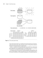
Example 3.11
A data cube is a lattice of cuboids. Suppose that you would like to create a data cube for
AllElectronics sales that contains the following: city, item, year, and sales in dollars. You
would like to be able to analyze the data, with queries such as the following:
“Compute the sum of sales, grouping by city and item.”
“Compute the sum of sales, grouping by city.”
“Compute the sum of sales, grouping by item.”
138 Chapter 3 Data Warehouse and OLAP Technology: An Overview
What is the total number of cuboids, or group-by’s, that can be computed for this

data cube? Taking the three attributes, city, item, and year, as the dimensions for the
data cube, and sales
in dollars as the measure, the total number of cuboids, or group-
by’s, that can be computed for this data cube is 2
3
= 8. The possible group-by’s are
the following: {(city, item, year), (city, item), (city, year), (item, year), (city), (item),
(year), ()}, where () means that the group-by is empty (i.e., the dimensions are not
grouped). These group-by’s form a lattice of cuboids for the data cube, as shown
in Figure 3.14. The base cuboid contains all three dimensions, city, item, and year.
It can return the total sales for any combination of the three dimensions. The apex
cuboid, or 0-D cuboid, refers to the case where the group-by is empty. It contains
the total sum of all sales. The base cuboid is the least generalized (most specific) of
the cuboids. The apex cuboid is the most generalized (least specific) of the cuboids,
and is often denoted as all. If we start at the apex cuboid and explore downward in
the lattice, this is equivalent to drilling down within the data cube. If we start at the
base cuboid and explore upward, this is akin to rolling up.
An SQL query containing no group-by, such as “compute the sum of total sales,” is a
zero-dimensional operation. An SQL query containing one group-by, such as “compute
the sum of sales, group by city,” is a one-dimensional operation. A cube operator on
n dimensions is equivalent to a collection of group by statements, one for each subset
(item)
(year)
(city)
()
(item, year)
(city, item, year)
(city, item)
(city, year)
O-D (apex) cuboid

1-D cuboids
2-D cuboids
3-D (base) cuboid
Figure 3.14 Lattice of cuboids, making up a 3-D data cube. Each cuboid represents a different group-by.
The base cuboid contains the three dimensions city, item, and year.
3.4 Data Warehouse Implementation 139
of the n dimensions. Therefore, the cube operator is the n-dimensional generalization of
the group by operator.
Based on the syntax of DMQL introduced in Section 3.2.3, the data cube in
Example 3.11 could be defined as
define cube sales
cube [city, item, year]: sum(sales in dollars)
For a cube with n dimensions, there are a total of 2
n
cuboids, including the base
cuboid. A statement such as
compute cube sales
cube
would explicitly instruct the system to compute the sales aggregate cuboids for all of the
eight subsets of the set {city, item, year}, including the empty subset. A cube computation
operator was first proposed and studied by Gray et al. [GCB
+
97].
On-line analytical processing may need to access different cuboids for different queries.
Therefore, it may seem like a good idea to compute all or at least some of the cuboids
in a data cube in advance. Precomputation leads to fast response time and avoids some
redundant computation. Most, if not all, OLAP products resort to some degree of pre-
computation of multidimensional aggregates.
A major challengerelated to this precomputation,however, is that the required storage
space may explode if all of the cuboids in a data cube are precomputed, especially when

the cube has many dimensions. The storage requirements are even more excessive when
many of the dimensions have associated concept hierarchies, each with multiple levels.
This problem is referred to as the curse of dimensionality. The extent of the curse of
dimensionality is illustrated below.
“How many cuboids are there in an n-dimensional data cube?” If there were no
hierarchies associated with each dimension, then the total number of cuboids for
an n-dimensional data cube, as we have seen above, is 2
n
. However, in practice,
many dimensions do have hierarchies. For example, the dimension time is usually not
explored at only one conceptual level, such as year, but rather at multiple conceptual
levels, such as in the hierarchy “day < month < quarter < year”. For an n-dimensional
data cube, the total number of cuboids that can be generated (including the cuboids
generated by climbing up the hierarchies along each dimension) is
Total number o f cuboids =
n
∏
i=1
(L
i
+ 1), (3.1)
where L
i
is the number of levels associated with dimension i. One is added to L
i
in
Equation (3.1) to include the virtual top level, all. (Note that generalizing to all is equiv-
alent to the removal of the dimension.) This formula is based on the fact that, at most,
one abstraction level in each dimension will appear in a cuboid. For example, the time
dimension as specified above has 4 conceptual levels, or 5 if we include the virtual level all.

If the cube has 10 dimensions and each dimension has 5 levels (including all), the total
number of cuboids that can be generated is 5
10
≈ 9.8 ×10
6
. The size of each cuboid
also depends on the cardinality (i.e., number of distinct values) of each dimension. For
example, if the AllElectronics branch in each city sold every item, there would be
140 Chapter 3 Data Warehouse and OLAP Technology: An Overview
|city| ×|item| tuples in the city-item group-by alone. As the number of dimensions,
number of conceptual hierarchies, or cardinality increases, the storage space required
for many of the group-by’s will grossly exceed the (fixed) size of the input relation.
By now, you probably realize that it is unrealistic to precompute and materialize all
of the cuboids that can possibly be generated for a data cube (or from a base cuboid). If
there are many cuboids, and these cuboids are large in size, a more reasonable option is
partial materialization, that is, to materialize only some of the possible cuboids that can
be generated.
Partial Materialization: Selected
Computation of Cuboids
There are three choices for data cube materialization given a base cuboid:
1. No materialization: Do not precompute any of the “nonbase” cuboids. This leads to
computing expensive multidimensional aggregates on the fly, which can be extremely
slow.
2. Full materialization: Precompute all of the cuboids. The resulting lattice of computed
cuboids is referred to as the full cube. This choice typically requires huge amounts of
memory space in order to store all of the precomputed cuboids.
3. Partial materialization: Selectively compute a proper subset of the whole set of possi-
ble cuboids. Alternatively, we may compute a subset of the cube, which contains only
those cells that satisfy some user-specified criterion, such as where the tuple count of
each cell isabovesome threshold.Wewill usethe term subcubeto refer to thelatter case,

where only some of the cells may be precomputed for various cuboids. Partial materi-
alization represents an interesting trade-off between storage space and response time.
The partial materialization of cuboids or subcubes should consider three factors:
(1) identify the subset of cuboids or subcubes to materialize; (2) exploit the mate-
rialized cuboids or subcubes during query processing; and (3) efficiently update the
materialized cuboids or subcubes during load and refresh.
The selection of the subset of cuboids or subcubes to materialize should take into
account the queries in the workload, their frequencies, and their accessing costs. In addi-
tion, itshouldconsider workload characteristics, thecostfor incremental updates,and the
total storage requirements. The selection must also consider the broad context of physical
database design, such as the generation and selection of indices. Several OLAP products
have adopted heuristic approaches for cuboid and subcube selection. Apopular approach
is to materialize theset ofcuboids onwhichother frequentlyreferencedcuboidsare based.
Alternatively, we can compute an iceberg cube, which is a data cube that stores only those
cube cells whose aggregate value (e.g., count) is above some minimum support threshold.
Another common strategy is to materialize a shell cube. This involves precomputing the
cuboids for only a small number of dimensions (such as 3 to 5) of a data cube. Queries
on additional combinations of the dimensions can be computed on-the-fly. Because our
3.4 Data Warehouse Implementation 141
aim in this chapter is to provide a solid introduction and overview of data warehousing
for data mining, we defer our detailed discussion of cuboid selection and computation
to Chapter 4, which studies data warehouse and OLAP implementation in greater depth.
Once the selected cuboids have been materialized, it is important to take advantage of
them during query processing. This involves several issues, such as how to determine the
relevant cuboid(s) from among the candidate materialized cuboids, how to use available
index structures on the materialized cuboids, and how to transform the OLAP opera-
tions onto the selected cuboid(s). These issues are discussed in Section 3.4.3 as well as in
Chapter 4.
Finally, during load and refresh, the materialized cuboids should be updated effi-
ciently. Parallelism and incremental update techniques for this operation should be

explored.
3.4.2 Indexing OLAP Data
To facilitate efficient data accessing, most data warehouse systems support index struc-
tures and materialized views (using cuboids). General methods to select cuboids for
materialization were discussed in the previous section. In this section, we examine how
to index OLAP data by bitmap indexing and join indexing.
The bitmap indexing method is popular in OLAP products because it allows quick
searching in data cubes. The bitmap index is an alternative representation of the
record
ID (RID) list. In the bitmap index for a given attribute, there is a distinct bit
vector, Bv, for each value v in the domain of the attribute. If the domain of a given
attribute consists of n values, then n bits are needed for each entry in the bitmap index
(i.e., there are n bit vectors). If the attribute has the value v for a given row in the data
table, then the bit representing that value is set to 1 in the corresponding row of the
bitmap index. All other bits for that row are set to 0.
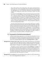
Example 3.12
Bitmap indexing. In the AllElectronics data warehouse, suppose the dimension item at the
top level has four values (representing item types): “home entertainment,” “computer,”
“phone,” and “security.” Each value (e.g., “computer”) is represented by a bit vector in
the bitmap index table for item. Suppose that the cube is stored as a relation table with
100,000 rows. Because the domain of item consists of four values, the bitmap index table
requires four bit vectors (or lists), each with 100,000 bits. Figure 3.15 shows a base (data)
table containing the dimensions item and city, and its mapping to bitmap index tables
for each of the dimensions.
Bitmap indexing is advantageous compared to hash and tree indices. It is especially
useful for low-cardinality domains because comparison, join, and aggregation opera-
tions are then reduced to bit arithmetic, which substantially reduces the processing time.
Bitmap indexing leads to significant reductions in space and I/O since a string of charac-
ters can be represented by a single bit. For higher-cardinality domains, the method can
be adapted using compression techniques.

The join indexing method gained popularity from its use in relational database query
processing. Traditional indexing maps the value in a given column to a list of rows having
142 Chapter 3 Data Warehouse and OLAP Technology: An Overview
RID item city
R1
R2
R3
R4
R5
R6
R7
R8
H
C
P
S
H
C
P
S
V
V
V
V
T
T
T
T
RID H C
R1

R2
R3
R4
R5
R6
R7
R8
1
0
0
0
1
0
0
0
0
1
0
0
0
1
0
0

P S
0
0
1
0
0

0
1
0
0
0
0
1
0
0
0
1
RID V T
R1
R2
R3
R4
R5
R6
R7
R8
1
1
1
1
0
0
0
0

0

0
0
0
1
1
1
1

Base table Item bitmap index table City bitmap index table
Note: H for “home entertainment, ” C for “computer, ” P for “phone, ” S for “security, ”
V for “Vancouver, ” T for “Toronto.”
Figure 3.15 Indexing OLAP data using bitmap indices.
that value. In contrast, join indexing registers the joinable rows of two relations from a
relational database. For example, if two relations R(RID, A) and S(B, SID) join on the
attributes A and B, then the join index record contains the pair (RID, SID), where RID
and SID are record identifiers from the R and S relations, respectively. Hence, the join
index records can identify joinable tuples without performing costly join operations. Join
indexing is especially useful for maintaining the relationship between a foreign key
3
and
its matching primary keys, from the joinable relation.
The star schema model of data warehouses makes join indexing attractive for cross-
table search, because the linkage between a fact table and its corresponding dimension
tables comprises the foreign key of the fact table and the primary key of the dimen-
sion table. Join indexing maintains relationships between attribute values of a dimension
(e.g., within a dimension table) and the corresponding rows in the fact table. Join indices
may span multiple dimensions to form composite join indices. We can use join indices
to identify subcubes that are of interest.
Example 3.13
Join indexing. In Example 3.4, we defined a star schema for AllElectronics of the form

“sales star [time, item, branch, location]: dollars sold = sum (sales in dollars)”. An exam-
ple of a join index relationship between the sales fact table and the dimension tables for
location and item is shown in Figure 3.16. For example, the “Main Street” value in the
location dimension table joins with tuples T57, T238, and T884 of the sales fact table.
Similarly, the “Sony-TV” value in the item dimension table joins with tuples T57 and
T459 of the sales fact table. The corresponding join index tables are shown in Figure 3.17.
3
A set of attributes in a relation schema that forms a primary key for another relation schema is called
a foreign key.
3.4 Data Warehouse Implementation 143
location
sales
item
Sony-TV
T57
T238
T459
Main Street
T884
Figure 3.16 Linkages between a sales fact table and dimension tables for location and item.
Figure 3.17 Join index tables based on the linkages between the sales fact table and dimension tables for
location and item shown in Figure 3.16.
Suppose that there are 360 time values, 100 items, 50 branches, 30 locations, and
10 million sales tuples in the sales
star data cube. If the sales fact table has recorded
sales for only 30 items, the remaining 70 items will obviously not participate in joins.
If join indices are not used, additional I/Os have to be performed to bring the joining
portions of the fact table and dimension tables together.
144 Chapter 3 Data Warehouse and OLAP Technology: An Overview
To further speed up query processing, the join indexing and bitmap indexing methods

can be integrated to form bitmapped join indices.
3.4.3 Efficient Processing of OLAP Queries
The purpose of materializing cuboids and constructing OLAP index structures is to
speed up query processing in data cubes. Given materialized views, query processing
should proceed as follows:
1. Determine which operations should be performed on the available cuboids: This
involves transforming any selection, projection, roll-up (group-by), and drill-down
operations specified in the query into corresponding SQL and/or OLAP operations.
For example, slicing and dicing a data cube may correspond to selection and/or pro-
jection operations on a materialized cuboid.
2. Determinetowhichmaterializedcuboid(s)therelevantoperationsshouldbeapplied:
This involves identifying all of the materialized cuboids that may potentially be used
to answer the query, pruning the above set using knowledge of “dominance” relation-
ships among the cuboids, estimating the costs of using the remaining materialized
cuboids, and selecting the cuboid with the least cost.
Example 3.14
OLAP query processing. Suppose that we define a data cube for AllElectronics of the form
“sales cube [time, item, location]: sum(sales in dollars)”. The dimension hierarchies used
are “day < month < quarter < year” for time, “item
name < brand < type” for item, and
“street < city < province or state < country” for location.
Suppose that the query to be processed is on {brand, province
or state}, with the
selection constant “year = 2004”. Also, suppose that there are four materialized cuboids
available, as follows:
cuboid 1: {year, item name, city}
cuboid 2: {year, brand, country}
cuboid 3: {year, brand, province or state}
cuboid 4: {item name, province or state} where year = 2004
“Which of the above four cuboids should be selected to process the query?” Finer-

granularity data cannot be generated from coarser-granularity data. Therefore, cuboid 2
cannot be used because country is a more general concept than province
or state.
Cuboids 1, 3, and 4 can be used to process the query because (1) they have the same set
or a superset of the dimensions in the query, (2) the selection clause in the query can
imply the selection in the cuboid, and (3) the abstraction levels for the item and loca-
tion dimensions in these cuboids are at a finer level than brand and province
or state,
respectively.
“How would the costs of each cuboid compare if used to process the query?” It is
likely that using cuboid 1 would cost the most because both item
name and city are
3.5 Data Warehouse Implementation 145
at a lower level than the brand and province
or state concepts specified in the query.
If there are not many year values associated with items in the cube, but there are
several item
names for each brand, then cuboid 3 will be smaller than cuboid 4, and
thus cuboid 3 should be chosen to process the query. However, if efficient indices
are available for cuboid 4, then cuboid 4 may be a better choice. Therefore, some
cost-based estimation is required in order to decide which set of cuboids should be
selected for query processing.
Because the storage model of a MOLAP server is an n-dimensional array, the front-
end multidimensional queries are mapped directly to server storage structures, which
provide direct addressing capabilities. The straightforward array representation of the
data cube has good indexing properties, but has poor storage utilization when the data
are sparse. For efficient storage and processing, sparse matrix and data compression tech-
niques should therefore be applied. The details of several such methods of cube compu-
tation are presented in Chapter 4.
The storage structures used by dense and sparse arrays may differ, making it advan-

tageous to adopt a two-level approach to MOLAP query processing: use array structures
for dense arrays, and sparse matrix structures for sparse arrays. The two-dimensional
dense arrays can be indexed by B-trees.
To process a query in MOLAP, the dense one- and two-dimensional arrays must first
be identified. Indices are then built to these arrays using traditional indexing structures.
The two-level approach increases storage utilization without sacrificing direct addressing
capabilities.
“Arethereanyotherstrategiesfor answeringqueriesquickly?”Some strategiesforanswer-
ing queries quicklyconcentrate on providing intermediate feedbackto theusers. Forexam-
ple,in on-lineaggregation, adatamining systemcandisplay“what itknowsso far”instead
of waiting until the query is fully processed. Such anapproximate answer to the given data
mining query is periodically refreshed and refined as the computation process continues.
Confidence intervals areassociated with each estimate, providing the user with additional
feedback regarding the reliability of the answer so far. This promotes interactivity with
the system—the user gains insight as to whether or not he or she is probing in the “right”
direction without having to wait until the end of the query. While on-line aggregation
does not improve the total time to answer a query, the overall data mining process should
be quicker due to the increased interactivity with the system.
Another approach is to employ top N queries. Suppose that you are interested in find-
ing only the best-selling items among the millions of items sold at AllElectronics. Rather
than waiting to obtain a list of all store items, sorted in decreasing order of sales, you
would like to see only the top N. Using statistics, query processing can be optimized to
return the top N items, rather than the whole sorted list. This results in faster response
time while helping to promote user interactivity and reduce wasted resources.
The goal of this section was to provide an overview of data warehouse implementa-
tion. Chapter 4 presents a more advanced treatment of this topic. It examines the efficient
computation of data cubes and processing of OLAP queries in greater depth, providing
detailed algorithms.
146 Chapter 3 Data Warehouse and OLAP Technology: An Overview
3.5

From Data Warehousing to Data Mining
“How do data warehousing and OLAP relate to data mining?” In this section, we study the
usage of data warehousing for information processing, analytical processing, and data
mining. We also introduce on-line analytical mining (OLAM), a powerful paradigm that
integrates OLAP with data mining technology.
3.5.1 Data Warehouse Usage
Data warehouses and data marts are used in a wide range of applications. Business
executives use the data in data warehouses and data marts to perform data analysis and
make strategic decisions. In many firms, data warehouses are used as an integral part
of a plan-execute-assess “closed-loop” feedback system for enterprise management.
Data warehouses are used extensively in banking and financial services, consumer
goods and retail distribution sectors, and controlled manufacturing, such as demand-
based production.
Typically, the longer a data warehouse has been in use, the more it will have evolved.
This evolution takes place throughout a number of phases. Initially, the data warehouse
is mainly used for generating reports and answering predefined queries. Progressively, it
is used to analyze summarized and detailed data, where the results are presented in the
form of reports and charts. Later, the data warehouse is used for strategic purposes, per-
forming multidimensional analysis and sophisticated slice-and-dice operations. Finally,
the data warehouse may be employed for knowledge discovery and strategic decision
making using data mining tools. In this context, the tools for data warehousing can be
categorized into access and retrieval tools, database reporting tools, data analysis tools, and
data mining tools.
Business users need to have the means to know what exists in the data warehouse
(through metadata), how to access the contents of the data warehouse, how to examine
the contents using analysis tools, and how to present the results of such analysis.
There are three kinds of data warehouse applications: information processing, analyt-
ical processing, and data mining:
Information processing supports querying, basic statistical analysis, and reporting
using crosstabs, tables, charts, or graphs. A current trend in data warehouse infor-

mation processing is to construct low-cost Web-based accessing tools that are then
integrated with Web browsers.
Analytical processing supports basic OLAP operations, including slice-and-dice,
drill-down, roll-up, and pivoting. It generally operates on historical data in both sum-
marized and detailed forms. The major strength of on-line analytical processing over
information processing is the multidimensional data analysis of data warehouse data.
Data mining supports knowledge discovery by finding hidden patterns and associa-
tions, constructing analytical models, performing classification and prediction, and
presenting the mining results using visualization tools.
3.5 From Data Warehousing to Data Mining 147
“How does data mining relate to information processing and on-line analytical
processing?” Information processing, based on queries, can finduseful information. How-
ever, answers to such queries reflect the information directly stored in databases or com-
putable by aggregate functions. They do not reflect sophisticated patterns or regularities
buried in the database. Therefore, information processing is not data mining.
On-line analytical processing comes a step closer to data mining because it can
derive information summarized at multiple granularities from user-specified subsets
of a data warehouse. Such descriptions are equivalent to the class/concept descrip-
tions discussed in Chapter 1. Because data mining systems can also mine generalized
class/concept descriptions, this raises some interesting questions: “Do OLAP systems
perform data mining? Are OLAP systems actually data mining systems?”
The functionalities of OLAP and data mining can be viewed as disjoint: OLAP is
a data summarization/aggregation tool that helps simplify data analysis, while data
mining allows the automated discovery of implicit patterns and interesting knowledge
hidden in large amounts of data. OLAP tools are targeted toward simplifying and
supporting interactive data analysis, whereas the goal of data mining tools is to
automate as much of the process as possible, while still allowing users to guide the
process. In this sense, data mining goes one step beyond traditional on-line analytical
processing.
An alternative and broader view of data mining may be adopted in which data

mining covers both data description and data modeling. Because OLAP systems can
present general descriptions of data from data warehouses, OLAP functions are essen-
tially for user-directed data summary and comparison (by drilling, pivoting, slicing,
dicing, and other operations). These are, though limited, data mining functionalities.
Yet according to this view, data mining covers a much broader spectrum than simple
OLAP operations because it performs not only data summary and comparison but
also association, classification, prediction, clustering, time-series analysis, and other
data analysis tasks.
Data mining is not confined to the analysis of data stored in data warehouses. It may
analyze data existing at more detailed granularities than the summarized data provided
in a data warehouse. It may also analyze transactional, spatial, textual, and multimedia
data that are difficult to model with current multidimensional database technology. In
this context, data mining covers a broader spectrum than OLAP with respect to data
mining functionality and the complexity of the data handled.
Because data mining involves more automated and deeper analysis than OLAP,
data mining is expected to have broader applications. Data mining can help busi-
ness managers find and reach more suitable customers, as well as gain critical
business insights that may help drive market share and raise profits. In addi-
tion, data mining can help managers understand customer group characteristics
and develop optimal pricing strategies accordingly, correct item bundling based
not on intuition but on actual item groups derived from customer purchase pat-
terns, reduce promotional spending, and at the same time increase the overall net
effectiveness of promotions.
148 Chapter 3 Data Warehouse and OLAP Technology: An Overview
3.5.2 From On-Line Analytical Processing to
On-Line Analytical Mining
In the field of data mining, substantial research has been performed for data mining on
various platforms, including transaction databases, relational databases,spatial databases,
text databases, time-series databases, flat files, data warehouses, and so on.
On-line analytical mining (OLAM) (also called OLAP mining) integrates on-line

analytical processing (OLAP) with data mining and mining knowledge in multidi-
mensional databases. Among the many different paradigms and architectures of data
mining systems, OLAM is particularly important for the following reasons:
High quality of data in data warehouses: Most data mining tools need to work
on integrated, consistent, and cleaned data, which requires costly data clean-
ing, data integration, and data transformation as preprocessing steps. A data
warehouse constructed by such preprocessing serves as a valuable source of high-
quality data for OLAP as well as for data mining. Notice that data mining may
also serve as a valuable tool for data cleaning and data integration as well.
Available information processing infrastructure surrounding data warehouses:
Comprehensive information processing and data analysis infrastructures have been
or will be systematically constructed surrounding data warehouses, which include
accessing, integration, consolidation, and transformation of multiple heterogeneous
databases, ODBC/OLE DB connections, Web-accessing and service facilities, and
reporting and OLAP analysis tools. It is prudent to make the best use of the
available infrastructures rather than constructing everything from scratch.
OLAP-based exploratory data analysis: Effective data mining needs exploratory
data analysis. A user will often want to traverse through a database, select por-
tions of relevant data, analyze them at different granularities, and present knowl-
edge/results in different forms. On-line analytical mining provides facilities for
data mining on different subsets of data and at different levels of abstraction,
by drilling, pivoting, filtering, dicing, and slicing on a data cube and on some
intermediate data mining results. This, together with data/knowledge visualization
tools, will greatly enhance the power and flexibility of exploratory data mining.
On-line selection of data mining functions: Often a user may not know what
kinds of knowledge she would like to mine. By integrating OLAP with multiple
data mining functions, on-line analytical mining provides users with the flexibility
to select desired data mining functions and swap data mining tasks dynamically.
Architecture for On-Line Analytical Mining
An OLAM server performs analytical mining in data cubes in a similar manner as an

OLAP server performs on-line analytical processing. An integrated OLAM and OLAP
architecture is shown in Figure 3.18, where the OLAM and OLAP servers both accept
user on-line queries (or commands) via a graphical user interface API and work with
the data cube in the data analysis via a cube API. A metadata directory is used to
3.5 From Data Warehousing to Data Mining 149
Graphical user interface API
Cube API
Database API
OLAP
engine
MDDB
Meta
data
Data
warehouse
Data filtering
Data integration
Data cleaning
Data integration
Filtering
OLAM
engine
Constraint-based
mining query
Mining result
Layer 4
user interface
Layer 3
OLAP/OLAM
Layer 2

multidimensional
database
Layer 1
data repository
Databases Databases
Figure 3.18 An integrated OLAM and OLAP architecture.
guide the access of the data cube. The data cube can be constructed by accessing
and/or integrating multiple databases via an MDDB API and/or by filtering a data
warehouse via a database API that may support OLE DB or ODBC connections.
Since an OLAM server may perform multiple data mining tasks, such as concept
description, association, classification, prediction, clustering, time-series analysis, and
so on, it usually consists of multiple integrated data mining modules and is more
sophisticated than an OLAP server.
150 Chapter 3 Data Warehouse and OLAP Technology: An Overview
Chapter 4 describes data warehouses on a finer level by exploring implementation
issues such as data cube computation, OLAP query answering strategies, and methods
of generalization. The chapters following it are devoted to the study of data min-
ing techniques. As we have seen, the introduction to data warehousing and OLAP
technology presented in this chapter is essential to our study of data mining. This
is because data warehousing provides users with large amounts of clean, organized,
and summarized data, which greatly facilitates data mining. For example, rather than
storing the details of each sales transaction, a data warehouse may store a summary
of the transactions per item type for each branch or, summarized to a higher level,
for each country. The capability of OLAP to provide multiple and dynamic views
of summarized data in a data warehouse sets a solid foundation for successful data
mining.
Moreover, we also believe that data mining should be a human-centered process.
Rather than asking a data mining system to generate patterns and knowledge automat-
ically, a user will often need to interact with the system to perform exploratory data
analysis.OLAP setsagood examplefor interactivedataanalysis andprovides thenecessary

preparations for exploratory data mining. Consider the discovery of association patterns,
for example. Instead of mining associations at a primitive (i.e., low) data level among
transactions, users should be allowed to specify roll-up operations along any dimension.
For example, a user may like to roll up on the item dimension to go from viewing the data
for particular TV sets that were purchased to viewing the brands of these TVs, such as
SONY or Panasonic. Users may also navigate from the transaction level to the customer
level or customer-type level in the search for interesting associations. Such an OLAP-
style of data mining is characteristic of OLAP mining. In our study of the principles of
data mining in this book, we place particular emphasis on OLAP mining, that is, on the
integration of data mining and OLAP technology.
3.6
Summary
A data warehouse is a subject-oriented, integrated, time-variant, and nonvolatile
collection of data organized in support of management decision making. Several
factors distinguish data warehouses from operational databases. Because the two
systems provide quite different functionalities and require different kinds of data,
it is necessary to maintain data warehouses separately from operational databases.
A multidimensional data model is typically used for the design of corporate data
warehouses and departmental data marts. Such a model can adopt a star schema,
snowflake schema, or fact constellation schema. The core of the multidimensional
model is the data cube, which consists of a large set of facts (or measures) and a
number of dimensions. Dimensions are the entities or perspectives with respect to
which an organization wants to keep records and are hierarchical in nature.
A data cube consists of a lattice of cuboids, each corresponding to a different
degree of summarization of the given multidimensional data.
3.6 Summary 151
Concept hierarchies organize the values of attributes or dimensions into gradual
levels of abstraction. They are useful in mining at multiple levels of abstraction.
On-line analytical processing (OLAP) can be performed in data warehouses/marts
using the multidimensional data model. Typical OLAP operations include roll-

up, drill-(down, across, through), slice-and-dice, pivot (rotate), as well as statistical
operations such as ranking and computing moving averages and growth rates.
OLAP operations can be implemented efficiently using the data cube structure.
Data warehouses often adopt a three-tier architecture. The bottom tier is a warehouse
database server, which is typically a relational database system. The middle tier is an
OLAP server, and the top tier is a client, containing query and reporting tools.
A data warehouse contains back-end tools and utilities for populating and refresh-
ing the warehouse. These cover data extraction, data cleaning, data transformation,
loading, refreshing, and warehouse management.
Data warehouse metadata are data defining the warehouse objects. A metadata
repository provides details regarding the warehouse structure, data history, the
algorithms used for summarization, mappings from the source data to warehouse
form, system performance, and business terms and issues.
OLAP servers may use relational OLAP (ROLAP), or multidimensional OLAP
(MOLAP), or hybrid OLAP (HOLAP). A ROLAP server uses an extended rela-
tional DBMS that maps OLAP operations on multidimensional data to standard
relational operations. A MOLAP server maps multidimensional data views directly
to array structures. A HOLAP server combines ROLAP and MOLAP. For example,
it may use ROLAP for historical data while maintaining frequently accessed data
in a separate MOLAP store.
Full materialization refers to the computation of all of the cuboids in the lattice defin-
ing a data cube. It typically requires an excessive amount of storage space, particularly
as the number of dimensions and size of associated concept hierarchies grow. This
problem is known as the curse of dimensionality. Alternatively, partial materializa-
tion is the selective computation of a subset of the cuboids or subcubes in the lattice.
For example, an iceberg cube is a data cube that stores only those cube cells whose
aggregate value (e.g., count) is above some minimum support threshold.
OLAP query processing can be made more efficient with the use of indexing tech-
niques. In bitmap indexing, each attribute has its own bitmap index table. Bitmap
indexing reduces join, aggregation, and comparison operations to bit arithmetic.

Join indexing registers the joinable rows of two or more relations from a rela-
tional database, reducing the overall cost of OLAP join operations. Bitmapped
join indexing, which combines the bitmap and join index methods, can be used
to further speed up OLAP query processing.
Data warehouses are used for information processing (querying and reporting), ana-
lytical processing (which allows users to navigate through summarized and detailed
152 Chapter 3 Data Warehouse and OLAP Technology: An Overview
data by OLAP operations), and data mining (which supports knowledge discovery).
OLAP-based data mining is referred to as OLAP mining, or on-line analytical mining
(OLAM), which emphasizes the interactive and exploratory nature of OLAP
mining.
Exercises
3.1 State why, for the integration of multiple heterogeneous information sources, many
companies in industry prefer the update-driven approach (which constructs and uses
data warehouses), rather than the query-driven approach (which applies wrappers and
integrators). Describe situations where the query-driven approach is preferable over
the update-driven approach.
3.2 Briefly compare the following concepts. You may use an example to explain your
point(s).
(a) Snowflake schema, fact constellation, starnet query model
(b) Data cleaning, data transformation, refresh
(c) Enterprise warehouse, data mart, virtual warehouse
3.3 Suppose that a data warehouse consists of the three dimensions time, doctor, and
patient, and the two measures count and charge, where charge is the fee that a doctor
charges a patient for a visit.
(a) Enumerate three classes of schemas that are popularly used for modeling data
warehouses.
(b) Draw a schema diagram for the above data warehouse using one of the schema
classes listed in (a).
(c) Starting with the base cuboid [day, doctor, patient], what specific OLAP operations

should be performed in order to list the total fee collected by each doctor in 2004?
(d) To obtain the same list, write an SQL query assuming the data are stored in a
relational database with the schema fee (day, month, year, doctor, hospital, patient,
count, charge).
3.4 Suppose that a data warehouse for Big University consists of the following four dimen-
sions: student, course, semester, and instructor, and two measures count and avg
grade.
When at the lowest conceptual level (e.g., for a given student, course, semester, and
instructor combination), the avg
grade measure stores the actual course grade of the
student. At higher conceptual levels, avg
grade stores the average grade for the given
combination.
(a) Draw a snowflake schema diagram for the data warehouse.
(b) Starting with the base cuboid [student, course, semester, instructor], what specific
OLAP operations (e.g., roll-up from semester to year) should one perform in order
to list the average grade of CS courses for each Big University student.