Data Mining Concepts and Techniques phần 9 pot

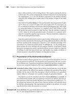
596 Chapter 10 Mining Object, Spatial, Multimedia, Text, and Web Data
via its closely related linkages in the class composition hierarchy. That is, in order to
discover interesting knowledge, generalization should be performed on the objects in the
class composition hierarchy that are closely related in semantics to the currently focused
class(es), but not on those that have only remote and rather weak semantic linkages.
10.1.5 Construction and Mining of Object Cubes
In an object database, data generalization and multidimensional analysis are not applied
to individual objects but to classes of objects. Since a set of objects in a class may share
many attributes and methods, and the generalization of each attribute and method may
apply a sequence of generalization operators, the major issue becomes how to make
the generalization processes cooperate among different attributes and methods in the
class(es).
“So, how can class-based generalization be performed for a large set of objects?” For class-
based generalization, the attribute-oriented induction method developed in Chapter 4 for
mining characteristics of relational databases can be extended to mine data character-
istics in object databases. Consider that a generalization-based data mining process can
be viewed as the application of a sequence of class-based generalization operators on
different attributes. Generalization can continue until the resulting class contains a small
number of generalized objects that can be summarized as a concise, generalized rule in
high-level terms. For efficient implementation, the generalization of multidimensional
attributes of a complex object class can be performed by examining each attribute (or
dimension), generalizing each attribute to simple-valued data, and constructing a mul-
tidimensional data cube, called an object cube. Once an object cube is constructed,
multidimensional analysis and data mining can be performed on it in a manner simi-
lar to that for relational data cubes.
Notice that from the application point of view, it is not always desirable to generalize
a set of values to single-valued data. Consider the attribute keyword, which may contain
a set of keywords describing a book. It does not make much sense to generalize this set
of keywords to one single value. In this context, it is difficult to construct an object cube
containing the keyword dimension. We will address some progress in this direction in
the next section when discussing spatial data cube construction. However, it remains a

challenging research issue to develop techniques for handling set-valued data effectively
in object cube construction and object-based multidimensional analysis.
10.1.6 Generalization-Based Mining of Plan Databases
by Divide-and-Conquer
To show how generalization can play an important role in mining complex databases,
we examine a case of mining significant patterns of successful actions in a plan database
using a divide-and-conquer strategy.
A plan consists of a variable sequence of actions. A plan database, or simply a
planbase, is a large collection of plans. Plan mining is the task of mining significant
10.1 Multidimensional Analysis and Descriptive Mining of Complex DataObjects 597
patterns or knowledge from a planbase. Plan mining can be used to discover travel
patterns of business passengers in an air flight database or to find significant patterns
from the sequences of actions in the repair of automobiles. Plan mining is differ-
ent from sequential pattern mining, where a large number of frequently occurring
sequences are mined at a very detailed level. Instead, plan mining is the extraction
of important or significant generalized (sequential) patterns from a planbase.
Let’s examine the plan mining process using an air travel example.
Example 10.4
An air flight planbase. Suppose that the air travel planbase shown in Table 10.1 stores
customer flight sequences, where each record corresponds to an action in a sequential
database, and a sequence of records sharing the same plan number is considered as one
plan with a sequence of actions. The columns departure and arrival specify the codes of
the airports involved. Table 10.2 stores information about each airport.
There could be many patterns mined from a planbase like Table 10.1. For example,
we may discover that most flights from cities in the Atlantic United States to Midwestern
cities have a stopover at ORD in Chicago, which could be because ORD is the princi-
pal hub for several major airlines. Notice that the airports that act as airline hubs (such
as LAX in Los Angeles, ORD in Chicago, and JFK in New York) can easily be derived
from Table 10.2 based on airport
size. However, there could be hundreds of hubs in a

travel database. Indiscriminate mining may result in a large number of “rules” that lack
substantial support, without providing a clear overall picture.
Table 10.1 A database of travel plans: a travel planbase.
plan# action# departure departure time arrival arrival time airline ···
1 1 ALB 800 JFK 900 TWA ···
1 2 JFK 1000 ORD 1230 UA ···
1 3 ORD 1300 LAX 1600 UA ···
1 4 LAX 1710 SAN 1800 DAL ···
2 1 SPI 900 ORD 950 AA ···
.
.
.
.
.
.
.
.
.
.
.
.
.
.
.
.
.
.
.
.
.

.
.
.
Table 10.2 An airport information table.
airport code city state region airport size ···
ORD Chicago Illinois Mid-West 100000 ···
SPI Springfield Illinois Mid-West 10000 ···
LAX Los Angeles California Pacific 80000 ···
ALB Albany New York Atlantic 20000 ···
.
.
.
.
.
.
.
.
.
.
.
.
.
.
.
.
.
.
598 Chapter 10 Mining Object, Spatial, Multimedia, Text, and Web Data
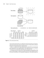
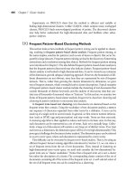
Figure 10.1 A multidimensional view of a database.
“So, how should we go about mining a planbase?” We would like to find a small

number of general (sequential) patterns that cover a substantial portion of the plans,
and then we can divide our search efforts based on such mined sequences. The key to
mining such patterns is to generalize the plans in the planbase to a sufficiently high level.
A multidimensional database model, such as the one shown in Figure 10.1 for the air
flight planbase, can be used to facilitate such plan generalization. Since low-level infor-
mation may never share enough commonality to form succinct plans, we should do the
following: (1) generalize the planbase in different directions using the multidimensional
model; (2) observe when the generalized plans share common, interesting, sequential
patterns with substantial support; and (3) derive high-level, concise plans.
Let’s examine this planbase. By combining tuples with the same plan number, the
sequences of actions (shown in terms of airport codes) may appear as follows:
ALB - JFK - ORD - LAX - SAN
SPI - ORD - JFK - SYR

10.1 Multidimensional Analysis and Descriptive Mining ofComplex Data Objects 599
Table 10.3 Multidimensional generalization of a planbase.
plan# loc seq size seq state seq region seq ···
1 ALB-JFK-ORD-LAX-SAN S-L-L-L-S N-N-I-C-C E-E-M-P-P ···
2 SPI-ORD-JFK-SYR S-L-L-S I-I-N-N M-M-E-E ···
.
.
.
.
.
.
.
.
.
.
.

.
.
.
.
.
.
.
Table 10.4 Merging consecutive, identical actions in plans.
plan# size seq state seq region seq ···
1 S-L
+
-S N
+
-I-C
+
E
+
-M-P
+
···
2 S-L
+
-S I
+
-N
+
M
+
-E
+

···
.
.
.
.
.
.
.
.
.
.
.
.
.
.
.
These sequences may look very different. However, they can be generalized in multiple
dimensions. When they are generalized based on the airport size dimension, we observe
some interesting sequential patterns, like S-L-L-S, where L represents a large airport (i.e.,
a hub), and S represents a relatively small regional airport, as shown in Table 10.3.
The generalization of a large number of air travel plans may lead to some rather gen-
eral but highly regular patterns. This is often the case if the merge and optional operators
are applied to the generalized sequences, where the former merges (and collapses) con-
secutive identical symbols into one using the transitive closure notation “+” to represent
a sequence of actions of the same type, whereas the latter uses the notation “[ ]” to indi-
cate that the object or action inside the square brackets “[ ]” is optional. Table 10.4 shows
the result of applying the merge operator to the plans of Table 10.3.
By merging and collapsing similar actions, we can derive generalized sequential pat-
terns, such as Pattern (10.1):
[S] −L

+
−[S] [98.5%] (10.1)
The pattern states that 98.5% of travel plans have the pattern [S] −L
+
−[S], where
[S] indicates that action S is optional, and L
+
indicates one or more repetitions of L.
In other words, the travel pattern consists of flying first from possibly a small airport,
hopping through one to many large airports, and finally reaching a large (or possibly, a
small) airport.
After a sequential pattern is found with sufficient support, it can be used to parti-
tion the planbase. We can then mine each partition to find common characteristics. For
example, from a partitioned planbase, we may find
flight(x, y) ∧airport
size(x,S) ∧airport size(y,L)⇒region(x) = region(y) [75%], (10.2)
600 Chapter 10 Mining Object, Spatial, Multimedia, Text, and Web Data
which means that for a direct flight from a small airport x to a large airport y, there is a
75% probability that x and y belong to the same region.
This example demonstrates a divide-and-conquer strategy, which first finds interest-
ing, high-level concise sequences of plans by multidimensional generalization of a
planbase, and then partitions the planbase based on mined patterns to discover the corre-
sponding characteristics of subplanbases. This mining approach can be applied to many
other applications. For example, in Weblog mining, we can study general access patterns
from the Web to identify popular Web portals and common paths before digging into
detailed subordinate patterns.
The plan mining technique can be further developed in several aspects. For instance,
a minimum support threshold similar to that in association rule mining can be used to
determine the level of generalization and ensure that a pattern covers a sufficient num-
ber of cases. Additional operators in plan mining can be explored, such as less

than.
Other variations include extracting associations from subsequences, or mining sequence
patterns involving multidimensional attributes—for example, the patterns involving
both airport size and location. Such dimension-combined mining also requires the gen-
eralization of each dimension to a high level before examinationof thecombined sequence
patterns.
10.2
Spatial Data Mining
A spatial database stores a large amount of space-related data, such as maps, prepro-
cessed remote sensing or medical imaging data, and VLSI chip layout data. Spatial
databases have many features distinguishing them from relational databases. They
carry topological and/or distance information, usually organized by sophisticated,
multidimensional spatial indexing structures that are accessed by spatial data access
methods and often require spatial reasoning, geometric computation, and spatial
knowledge representation techniques.
Spatial data mining refers to the extraction of knowledge, spatial relationships, or
other interesting patterns not explicitly stored in spatial databases. Such mining demands
an integration of data mining with spatial database technologies. It can be used for under-
standing spatial data, discovering spatial relationships and relationships between spatial
and nonspatial data, constructing spatial knowledge bases,reorganizing spatial databases,
and optimizing spatial queries. It is expected to have wide applications in geographic
information systems, geomarketing, remote sensing, image database exploration, medi-
cal imaging, navigation, traffic control, environmental studies, and many other areas
where spatial data are used. A crucial challenge to spatial data mining is the exploration
of efficient spatial data mining techniques due to the huge amount of spatial data and the
complexity of spatial data types and spatial access methods.
“What about using statistical techniques for spatial data mining?” Statistical spatial data
analysis has been a popular approach to analyzing spatial data and exploring geographic
information. The term geostatistics is often associated with continuous geographic space,
10.2 Spatial Data Mining 601

whereas the term spatial statistics is often associated with discrete space. In a statistical
model that handles nonspatial data, one usually assumes statistical independence among
different portions of data. However, different from traditional data sets, there is no such
independence among spatially distributed databecause in reality, spatial objects are often
interrelated, or more exactly spatially co-located, in the sense that the closer the two objects
are located, the more likely they share similar properties. For example, nature resource,
climate, temperature, and economic situations are likely to be similar in geographically
closely located regions. People even consider this as the firstlaw of geography: “Everything
is related to everything else, but nearby things are more related than distant things.” Such
a property of close interdependency across nearby space leads to the notion of spatial
autocorrelation. Based on this notion, spatial statistical modeling methods have been
developed with good success. Spatial data mining will further develop spatial statistical
analysis methods and extend them for huge amounts of spatial data, with more emphasis
on efficiency, scalability, cooperation with database and data warehouse systems,
improved user interaction, and the discovery of new types of knowledge.
10.2.1 Spatial Data Cube Construction and Spatial OLAP
“Can we construct a spatial data warehouse?” Yes, as with relational data, we can integrate
spatial data to construct a data warehouse that facilitates spatial data mining. A spatial
data warehouse is a subject-oriented, integrated, time-variant, and nonvolatile collection
of both spatial and nonspatial data in support of spatial data mining and spatial-data-
related decision-making processes.
Let’s look at the following example.
Example 10.5
Spatial data cube and spatial OLAP. There are about 3,000 weather probes distributed in
British Columbia (BC), Canada, each recording daily temperature and precipitation for
a designated small area and transmitting signals to a provincial weather station. With a
spatial data warehouse that supports spatial OLAP, a user can view weather patterns on a
map by month, by region, and by different combinations of temperature and precipita-
tion, and can dynamically drill down or roll up along any dimension to explore desired
patterns, such as “wet and hot regions in the Fraser Valley in Summer 1999.”

There are several challenging issues regarding the construction and utilization of
spatial data warehouses. The first challenge is the integration of spatial data from het-
erogeneous sources and systems. Spatial data are usually stored in different industry
firms and government agencies using various data formats. Data formats are not only
structure-specific (e.g., raster- vs. vector-based spatial data, object-oriented vs. relational
models, different spatial storage and indexing structures), but also vendor-specific (e.g.,
ESRI, MapInfo, Intergraph). There has been a great deal of work on the integration and
exchange of heterogeneous spatial data, which has paved the way for spatial data inte-
gration and spatial data warehouse construction.
The second challenge is the realization of fastand flexible on-line analytical processing
in spatial data warehouses. The star schema model introduced in Chapter 3 is a good
602 Chapter 10 Mining Object, Spatial, Multimedia, Text, and Web Data
choice for modeling spatial data warehouses because it provides a concise and organized
warehouse structure and facilitates OLAP operations. However, in a spatial warehouse,
both dimensions and measures may contain spatial components.
There are three types of dimensions in a spatial data cube:
A nonspatial dimension contains only nonspatial data. Nonspatial dimensions
temperature and precipitation can be constructed for the warehouse in Example 10.5,
since each contains nonspatial data whose generalizations are nonspatial (such as
“hot” for temperature and “wet” for precipitation).
A spatial-to-nonspatial dimension is a dimension whose primitive-level data are spa-
tial but whose generalization, starting at a certain high level, becomes nonspatial. For
example, the spatial dimension city relays geographic data for the U.S. map. Suppose
that the dimension’s spatial representation of, say, Seattle is generalized to the string
“pacific
northwest.” Although “pacific northwest” is a spatial concept, its representa-
tion is not spatial (since, in our example, it is a string). It therefore plays the role of a
nonspatial dimension.
A spatial-to-spatial dimension is adimension whose primitive level andall of its high-
level generalized data are spatial. For example, the dimension equi

temperature region
contains spatial data, as do all of its generalizations, such as with regions covering
0-5
degrees (Celsius), 5-10 degrees, and so on.
We distinguish two types of measures in a spatial data cube:
A numerical measure contains only numerical data. For example, one measure in a
spatial data warehouse could be the monthly
revenue of a region, so that a roll-up may
compute the total revenue by year, by county, and so on. Numerical measures can be
further classified into distributive, algebraic, and holistic, as discussed in Chapter 3.
A spatial measure contains a collection of pointers to spatial objects. For example,
in a generalization (or roll-up) in the spatial data cube of Example 10.5, the regions
with the same range of temperature and precipitation will be grouped into the same
cell, and the measure so formed contains a collection of pointers to those regions.
A nonspatial data cube contains only nonspatial dimensions and numerical measures.
If a spatial data cube contains spatial dimensions but no spatial measures, its OLAP
operations, such as drilling or pivoting, can be implemented in a manner similar to that
for nonspatial data cubes.
“But what if I need to use spatial measures in a spatial data cube?” This notion raises
some challenging issues on efficient implementation, as shown in the following example.
Example 10.6
Numerical versus spatial measures. A star schema for the BC weather warehouse of
Example 10.5 is shown in Figure 10.2. It consists of four dimensions: region temperature,
time, and precipitation, and three measures: region
map, area, and count. A concept hier-
archy for each dimension can be created by users or experts, or generated automatically
10.2 Spatial Data Mining 603
by data clustering analysis. Figure 10.3 presents hierarchies for each of the dimensions
in the BC
weather warehouse.

Of the three measures, area and count are numerical measures that can be computed
similarly as for nonspatial data cubes; region
map is a spatial measure that represents a
collection of spatial pointers to the corresponding regions. Since different spatial OLAP
operations result in different collections of spatial objects in region
map, it is a major
challenge to compute the merges of a large number of regions flexibly and dynami-
cally. For example, two different roll-ups on the BC weather map data (Figure 10.2) may
produce two different generalized region maps, as shown in Figure 10.4, each being the
result of merging a large number of small (probe) regions from Figure 10.2.
Figure 10.2 A star schema of the BC weather spatial data warehouse and corresponding BC weather
probes map.
region
name dimension: time dimension:
probe
location < district < city < region hour < day < month < season
< province
temperature dimension: precipitation dimension:
(cold, mild, hot) ⊂ all(temperature) (dry, fair, wet) ⊂ all(precipitation)
(below
−20, −20 −11, −10 0) ⊂ cold (0 0.05, 0.06 0.2) ⊂ dry
(0 10, 11 15, 16 20) ⊂ mild (0.2 0.5, 0.6 1.0, 1.1 1.5) ⊂ fair
(20 25, 26 30, 31 35, above
35) ⊂ hot (1.5 2.0, 2.1 3.0, 3.1 5.0, above 5.0)
⊂ wet
Figure 10.3 Hierarchies for each dimension of the BC weather data warehouse.
604 Chapter 10 Mining Object, Spatial, Multimedia, Text, and Web Data
Figure 10.4 Generalized regions after different roll-up operations.
“Can we precompute all of the possible spatial merges and store them in the corresponding
cuboid cells of a spatial data cube?” The answer is—probably not. Unlike a numerical mea-

sure where each aggregated value requires only a few bytes of space, a merged region map
of BC may require multi-megabytes of storage. Thus, we face a dilemma in balancing the
cost of on-line computation and the space overhead of storing computed measures: the
substantial computation cost for on-the-fly computation of spatial aggregations calls for
precomputation, yet substantial overhead for storing aggregated spatial values discour-
ages it.
There are at least three possible choices in regard to the computation of spatial
measures in spatial data cube construction:
Collect and store the corresponding spatial object pointers but do not perform precom-
putation of spatial measures in the spatial data cube. This can be implemented by
storing, in the corresponding cube cell, a pointer to a collection of spatial object point-
ers, andinvoking and performing the spatial merge (or other computation) of the cor-
responding spatial objects, when necessary, on the fly. This method is a good choice if
only spatial display is required (i.e., no real spatial merge has to be performed), or if
there are not many regions to be merged in any pointer collection (so that the on-line
merge is not very costly), or if on-line spatial merge computation is fast (recently,
some efficient spatial merge methods have been developed for fast spatial OLAP).
Since OLAP results are often used for on-line spatial analysis and mining, it is still
recommended to precompute some of the spatially connected regions to speed up
such analysis.
Precompute and store a rough approximation of the spatial measures in the spatial data
cube. This choice is good for a rough view or coarse estimation of spatial merge results
under the assumption that it requires little storage space. For example, a minimum
boundingrectangle(MBR),representedby twopoints,canbetakenasaroughestimate
10.2 Spatial Data Mining 605
of a merged region. Such a precomputed result is small and can be presented quickly
to users. If higher precision is needed for specific cells, the application can either fetch
precomputed high-quality results, if available, or compute them on the fly.
Selectively precompute some spatial measures in the spatial data cube. This can be a
smart choice. The question becomes, “Which portion of the cube should be selected

for materialization?” The selection can be performed at the cuboid level, that is, either
precompute and store each set of mergeable spatial regions for each cell of a selected
cuboid, or precompute none if the cuboid is not selected. Since a cuboid usually con-
sists of a large number of spatial objects, it may involve precomputation and storage
of a large number of mergeable spatial objects, some of which may be rarely used.
Therefore, it is recommended to perform selection at a finer granularity level: exam-
ining each group of mergeable spatial objects in a cuboid to determine whether such
a merge should be precomputed. The decision should be based on the utility (such as
access frequency or access priority), shareability of merged regions, and the balanced
overall cost of space and on-line computation.
With efficient implementation of spatial data cubes and spatial OLAP, generalization-
based descriptive spatial mining, such as spatial characterization and discrimination, can
be performed efficiently.
10.2.2 Mining Spatial Association and Co-location Patterns
Similar to the mining of association rules in transactional and relational databases,
spatial association rules can be mined in spatial databases. A spatial association rule is of
the form A ⇒ B [s%, c%], where A and B are sets of spatial or nonspatial predicates, s%
is the support of the rule, and c% is the confidence of the rule. For example, the following
is a spatial association rule:
is
a(X,“school”) ∧close to(X, “sports center”) ⇒ close to(X, “park”) [0.5%,80%].
This rule states that 80% of schools that are close to sports centers are also close to
parks, and 0.5% of the data belongs to such a case.
Various kinds of spatial predicates can constitute a spatial association rule. Examples
include distance information (such as close
to and far away), topological relations (like
intersect, overlap, and disjoint), and spatial orientations (like left of and west of).
Sincespatialassociation mining needstoevaluatemultiplespatial relationships among
a large number of spatial objects, the process could be quite costly. An interesting mining
optimization method called progressive refinement can be adopted in spatial association

analysis. The method first mines large data sets roughly using a fast algorithm and then
improves the quality of mining in a pruned data set using a more expensive algorithm.
To ensure that the pruned data set covers the complete set of answers when applying
the high-quality data mining algorithms at a laterstage, an important requirement for the
rough mining algorithm applied in the early stage is the superset coverage property: that
is, it preserves all of the potential answers. In other words, it should allow a false-positive
606 Chapter 10 Mining Object, Spatial, Multimedia, Text, and Web Data
test, which might include some data sets that do not belong to the answer sets, but it
should not allow a false-negative test, which might exclude some potential answers.
For mining spatial associations related to the spatial predicate close
to, we can first
collect the candidates that pass the minimum support threshold by
Applying certain rough spatial evaluation algorithms, for example, using an MBR
structure (which registers only two spatial points rather than a set of complex
polygons), and
Evaluating the relaxed spatial predicate, g close to, which is a generalized close to
covering a broader context that includes close to, touch, and intersect.
If two spatial objects are closely located, their enclosing MBRs must be closely located,
matching g close to. However, the reverse is not always true: if the enclosing MBRs are
closely located, the two spatial objects may or may not be located so closely. Thus, the
MBR pruning is a false-positive testing tool for closeness: only those that pass the rough
test need to be further examined using more expensive spatial computation algorithms.
With thispreprocessing, only thepatternsthat are frequent at theapproximation levelwill
need to be examined by more detailed and finer, yet more expensive, spatial computation.
Besides mining spatial association rules, one may like to identify groups of particular
features that appear frequently close to each other in a geospatial map. Such a problem
is essentially the problem of mining spatial co-locations. Finding spatial co-locations
can be considered as a special case of mining spatial associations. However, based on the
property of spatial autocorrelation, interesting features likely coexist in closely located
regions. Thus spatial co-location can be just what one really wants to explore. Efficient

methods can be developed for mining spatial co-locations by exploring the methodolo-
gies like Aprori and progressive refinement, similar to what has been done for mining
spatial association rules.
10.2.3 Spatial Clustering Methods
Spatial dataclustering identifies clusters, or densely populated regions, according to some
distance measurement in a large, multidimensional data set. Spatial clustering methods
were thoroughly studied in Chapter 7 since cluster analysis usually considers spatial data
clustering in examples and applications. Therefore, readers interested in spatial cluster-
ing should refer to Chapter 7.
10.2.4 Spatial Classification and Spatial Trend Analysis
Spatial classification analyzes spatial objects to derive classification schemes in relevance
to certain spatial properties, such as the neighborhood of a district, highway, or river.
Example 10.7
Spatial classification. Suppose that you would like to classify regions in a province into
rich versus poor according to the average family income. In doing so, you would like
to identify the important spatial-related factors that determine a region’s classification.
10.3 Multimedia Data Mining 607
Many properties are associated with spatial objects, such as hosting a university,
containing interstate highways, being near a lake or ocean, and so on. These prop-
erties can be used for relevance analysis and to find interesting classification schemes.
Such classification schemes may be represented in the form of decision trees or rules,
for example, as described in Chapter 6.
Spatial trend analysis deals with another issue: the detection of changes and trends
along a spatial dimension. Typically, trend analysis detects changes with time, such as the
changes of temporal patterns in time-series data. Spatial trend analysis replaces time with
spaceand studies thetrendofnonspatial or spatial datachanging with space. For example,
we may observe the trend of changes in economic situation when moving away from the
center of a city, or the trend of changes of the climate or vegetation with the increasing
distance from an ocean. For such analyses, regression and correlation analysis methods
are often applied by utilization of spatial data structures and spatial access methods.

There are also many applications where patterns are changing with both space and
time. For example, traffic flows on highways and in cities are both time and space related.
Weather patterns are also closely related to both time and space. Although there have
been a few interesting studies on spatial classification and spatial trend analysis, the inves-
tigation of spatiotemporal data mining is still in its early stage. More methods and appli-
cations of spatial classification and trend analysis, especially those associated with time,
need to be explored.
10.2.5 Mining Raster Databases
Spatial database systems usually handle vector data that consist of points, lines, polygons
(regions), and their compositions, such as networks or partitions. Typical examples of
such data include maps, design graphs, and 3-D representations of the arrangement of
the chains of protein molecules. However, a huge amount of space-related data are in
digital raster (image) forms, such as satellite images, remote sensing data, and computer
tomography. It is important to explore datamining inraster or image databases.Methods
for mining raster and image data are examined in the following section regarding the
mining of multimedia data.
10.3
Multimedia Data Mining
“What is a multimedia database?” A multimedia database system stores and manages a
large collection of multimedia data, such as audio, video, image, graphics, speech, text,
document, and hypertext data, which contain text, text markups, and linkages. Multi-
media database systems are increasingly common owing to the popular use of audio-
video equipment, digital cameras, CD-ROMs, and the Internet. Typical multimedia
database systems include NASA’s EOS (Earth Observation System), various kinds of
image and audio-video databases, and Internet databases.
In this section, our study of multimedia data mining focuses on image data mining.
Mining text data and mining the World Wide Web are studied in the two subsequent
608 Chapter 10 Mining Object, Spatial, Multimedia, Text, and Web Data
sections. Here we introduce multimedia data mining methods, including similarity
search in multimedia data, multidimensional analysis, classification and prediction

analysis, and mining associations in multimedia data.
10.3.1 Similarity Search in Multimedia Data
“When searching for similarities in multimedia data, can we search on either the data
description or the data content?” That is correct. For similarity searching in multimedia
data, we consider two main families of multimedia indexing and retrieval systems: (1)
description-based retrieval systems, which build indices and perform object retrieval
based on image descriptions, such as keywords, captions, size, and time of creation;
and (2) content-based retrieval systems, which support retrieval based on the image
content, such as color histogram, texture, pattern, image topology, and the shape of
objects and their layouts and locations within the image. Description-based retrieval
is labor-intensive if performed manually. If automated, the results are typically of
poor quality. For example, the assignment of keywords to images can be a tricky and
arbitrary task. Recent development of Web-based image clustering and classification
methods has improved the quality of description-based Web image retrieval, because
imagesurrounded text information as well as Web linkage information can be used
to extract proper description and group images describing a similar theme together.
Content-based retrieval uses visual features to index images and promotes object
retrieval based on feature similarity, which is highly desirable in many applications.
In a content-based image retrieval system, there are often two kinds of queries: image-
sample-based queries and image feature specification queries. Image-sample-based queries
find all of the images that are similar to the given image sample. This search compares
the feature vector (or signature) extracted from the sample with the feature vectors of
images that have already been extracted and indexed in the image database. Based on
this comparison, images that are close to the sample image are returned. Image feature
specification queries specify or sketch image features like color, texture, or shape, which
are translated into a feature vector to be matched with the feature vectors of the images in
the database.Content-based retrieval haswide applications, including medical diagnosis,
weather prediction, TV production, Web search engines for images, and e-commerce.
Some systems, such as QBIC (Query By Image Content), support both sample-based and
image feature specification queries. There are also systems that support both content-

based and description-based retrieval.
Several approaches have been proposed and studied for similarity-based retrieval in
image databases, based on image signature:
Color histogram–based signature: In this approach, the signature of an image
includes color histograms based on the color composition of an image regardless of
its scale or orientation. This method does not contain any information about shape,
image topology, or texture. Thus, two images with similar color composition but
that contain very different shapes or textures may be identified as similar, although
they could be completely unrelated semantically.
10.3 Multimedia Data Mining 609
Multifeature composed signature: In this approach, the signature of an image
includes a composition of multiple features: color histogram, shape, image topol-
ogy, and texture. The extracted image features are stored as metadata, and images
are indexed based on such metadata. Often, separate distance functions can be
defined for each feature and subsequently combined to derive the overall results.
Multidimensional content-based search often uses one or a few probe features to
search for images containing such (similar) features. It can therefore be used to
search for similar images. This is the most popularly used approach in practice.
Wavelet-based signature: This approach uses the dominant wavelet coefficients of an
image as its signature. Wavelets capture shape, texture, and image topology informa-
tion in a single unified framework.
1
This improves efficiency and reduces the need
for providing multiple search primitives (unlike the second method above). How-
ever, since this method computes a single signature for an entire image, it may fail to
identify images containing similar objects where the objects differ in location or size.
Wavelet-based signature with region-based granularity: In this approach, the com-
putation and comparison of signatures are at the granularity of regions, not the entire
image. This is based on the observation that similar images may contain similar
regions, but a region in one image could be a translation or scaling of a matching

region in the other. Therefore, a similarity measure between the query image Q and
a target image T can be defined in terms of the fraction of the area of the two images
covered by matching pairs of regions from Q and T. Such a region-based similar-
ity search can find images containing similar objects, where these objects may be
translated or scaled.
10.3.2 Multidimensional Analysis of Multimedia Data
“Can we construct a data cube for multimedia data analysis?” To facilitate the multidimen-
sional analysis of large multimedia databases,multimedia data cubes can be designed and
constructed in a manner similar to that for traditional data cubes from relational data.
A multimedia data cube can contain additional dimensions and measures for multime-
dia information, such as color, texture, and shape.
Let’s examine a multimedia data mining system prototype called MultiMediaMiner,
which extends the DBMiner system by handling multimedia data. The example database
tested in the MultiMediaMiner system is constructed as follows. Each image contains
two descriptors: a feature descriptor and a layout descriptor. The original image is not
stored directly in the database; only its descriptors are stored. The description informa-
tion encompasses fields like image file name, image URL, image type (e.g., gif, tiff, jpeg,
mpeg, bmp, avi), alist of all known Web pages referring to the image (i.e.,parent URLs),a
list of keywords, and a thumbnail used by the user interface for image and video brows-
ing. The feature descriptor is a set of vectors for each visual characteristic. The main
1
Wavelet analysis was introduced in Section 2.5.3.
610 Chapter 10 Mining Object, Spatial, Multimedia, Text, and Web Data
vectors are a color vector containing the color histogram quantized to 512 colors (8 ×
8×8 for R×G×B), an MFC(Most Frequent Color) vector, and an MFO (Most Frequent
Orientation) vector. The MFC and MFO contain five color centroids and five edge ori-
entation centroids for the five most frequent colors and five most frequent orientations,
respectively. The edge orientations used are 0
◦
, 22.5

◦
, 45
◦
, 67.5
◦
, 90
◦
, and so on. The
layout descriptor contains a color layout vector and an edge layout vector. Regardless
of their original size, all images are assigned an 8×8 grid. The most frequent color for
each of the 64 cells is stored in the color layout vector, and the number of edges for each
orientation in each of the cells is stored in the edge layout vector. Other sizes of grids,
like 4×4, 2 ×2, and 1×1, can easily be derived.
The Image Excavator component of MultiMediaMiner uses image contextual infor-
mation, like HTML tags in Web pages, to derive keywords. By traversing on-line direc-
tory structures, like the Yahoo! directory, it is possible to create hierarchies of keywords
mapped onto the directories in which the image was found. These graphs are used as
concept hierarchies for the dimension keyword in the multimedia data cube.
“What kind of dimensions can a multimedia data cube have?” A multimedia data
cube can have many dimensions. The following are some examples: the size of the
image or video in bytes; the width and height of the frames (or pictures), constituting
two dimensions; the date on which the image or video was created (or last modified);
the format type of the image or video; the frame sequence duration in seconds;
the image or video Internet domain; the Internet domain of pages referencing the
image or video (parent URL); the keywords; a color dimension; an edge-orientation
dimension; and so on. Concept hierarchies for many numerical dimensions may be
automatically defined. For other dimensions, such as for Internet domains or color,
predefined hierarchies may be used.
The construction of a multimedia data cube will facilitate multidimensional analysis
of multimedia data primarily based onvisual content, andthe mining ofmultiple kindsof

knowledge, including summarization, comparison, classification, association,
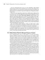
and clustering. The Classifier module of MultiMediaMiner and its output are presented
in Figure 10.5.
The multimedia data cube seems to be an interesting model for multidimensional
analysis of multimedia data. However, we should note that it is difficult to implement
a data cube efficiently given a large number of dimensions. This curse of dimensiona-
lity is especially serious in the case of multimedia data cubes. We may like to model
color, orientation, texture, keywords, and so on, as multiple dimensions in a multimedia
data cube. However, many of these attributes are set-oriented instead of single-valued.
For example, one image may correspond to a set of keywords. It may contain a set of
objects, each associated with a set of colors. If we use each keyword as a dimension or
each detailed color as a dimension in the design of the data cube, it will create a huge
number of dimensions. On the other hand, not doing so may lead to the modeling of an
image at a rather rough, limited, and imprecise scale. More research is needed on how
to design a multimedia data cube that may strike a balance between efficiency and the
power of representation.
10.3 Multimedia Data Mining 611
Figure 10.5 An output of the Classifier module of MultiMediaMiner.
10.3.3 Classification and Prediction Analysis of Multimedia Data
Classification and predictive modeling have been used for miningmultimedia data, espe-
cially in scientific research, such as astronomy, seismology, and geoscientific research. In
general, all of the classification methods discussed in Chapter 6 can be used in image
analysis and pattern recognition. Moreover, in-depth statistical pattern analysis methods
are popular for distinguishing subtle features and building high-quality models.
Example 10.8
Classification and prediction analysis of astronomy data. Taking sky images that have
been carefully classified by astronomers as the training set, we can construct models
for the recognition of galaxies, stars, and other stellar objects, based on properties like
magnitudes, areas, intensity, image moments, and orientation. A large number of sky
images taken by telescopes or space probes can then be tested against the constructed

models in order to identify new celestial bodies. Similar studies have successfully been
performed to identify volcanoes on Venus.
Data preprocessing is important when mining image data and can include data
cleaning, data transformation, andfeature extraction. Aside from standardmethods used
in pattern recognition, such as edge detection and Hough transformations, techniques
612 Chapter 10 Mining Object, Spatial, Multimedia, Text, and Web Data
can be explored, such as the decomposition of images to eigenvectors or the adoption
of probabilistic models to deal with uncertainty. Since the image data are often in huge
volumes and may require substantial processing power, parallel and distributed process-
ing are useful. Image data mining classification and clustering are closely linked to image
analysis and scientific data mining, and thus many image analysis techniques and scien-
tific data analysis methods can be applied to image data mining.
The popular use of the World Wide Web has made the Web a rich and gigantic reposi-
tory of multimedia data. The Web not only collects a tremendous number of photos, pic-
tures, albums, and video images in the form of on-line multimedia libraries, but also has
numerous photos, pictures, animations, and other multimedia forms on almost every
Web page. Such pictures and photos, surrounded by text descriptions, located at the
different blocks of Web pages, or embedded inside news or text articles, may serve rather
different purposes, such as forming an inseparable component of the content, serving as
an advertisement, or suggesting an alternative topic. Furthermore, these Web pages are
linked with other Web pages in a complicated way. Such text, image location, and Web
linkage information, if used properly, may help understand the contents of the text or
assist classification and clustering of images on the Web. Data mining by making good
use of relative locations and linkages among images, text, blocks within a page, and page
links on the Web becomes an important direction in Web data analysis, which will be
further examined in Section 10.5 on Web mining.
10.3.4 Mining Associations in Multimedia Data
“What kinds of associations can be mined in multimedia data?” Association rules involving
multimedia objects can be mined in image and video databases. At least three categories
can be observed:

Associations between image content andnonimage content features: A rule like “If at
least 50% of the upper part of the picture is blue, then it is likely to represent sky” belongs
to this category since it links the image content to the keyword sky.
Associations among image contents that are not related to spatial relationships: A
rule like “If a picture contains two blue squares, then it is likely to contain one red circle
as well” belongs to this category since the associations are all regarding image contents.
Associations among image contents related to spatial relationships: A rule like “If
a red triangle is between two yellow squares, then it is likely a big oval-shaped object
is underneath” belongs to this category since it associates objects in the image with
spatial relationships.
To mine associations among multimedia objects, we can treat each image as a tran-
saction and find frequently occurring patterns among different images.
“What are the differences between mining association rules in multimedia databases
versus in transaction databases?” There are some subtle differences. First, an image may
contain multiple objects, each with many features such as color, shape, texture,
10.3 Multimedia Data Mining 613
keyword, and spatial location, so there could be many possible associations. In many
cases, a feature may be considered as the same in two images at a certain level of resolu-
tion, but different at a finer resolution level. Therefore, it is essential to promote a pro-
gressive resolution refinement approach. That is, we can first mine frequently occurring
patterns at a relatively rough resolution level, and then focus only on those that have
passed the minimum support threshold when mining at a finer resolution level. This is
because the patterns that are not frequent at a rough level cannot be frequent at finer
resolution levels. Such a multiresolution mining strategy substantially reduces the over-
all data mining cost without loss of the quality and completeness of data mining results.
This leads to an efficient methodology for mining frequent itemsets and associations in
large multimedia databases.
Second, because a picture containing multiple recurrent objects is an important
feature in image analysis, recurrence of the same objects should not be ignored in asso-
ciation analysis. For example, a picture containing two golden circles is treated quite

differently from that containing only one. This is quite different from that in a transac-
tion database, where the fact that a person buys one gallon of milk or two may often be
treated the same as “buys
milk.” Therefore, the definition of multimedia association and
its measurements, such as support and confidence, should be adjusted accordingly.
Third, there often exist important spatial relationships among multimedia objects,
such as above, beneath, between, nearby, left-of, and so on. These features are very use-
ful for exploring object associations and correlations. Spatial relationships together with
other content-based multimedia features, such as color, shape, texture, and keywords,
may form interesting associations. Thus, spatial data mining methods and properties of
topological spatial relationships become important for multimedia mining.
10.3.5 Audio and Video Data Mining
Besides still images, an incommensurable amount of audiovisual information is becom-
ing available in digital form, in digital archives, on the World Wide Web, inbroadcast data
streams, and in personal and professional databases. This amount is rapidly growing.
There are great demands for effective content-based retrieval and data mining methods
for audio and video data. Typical examples include searching for and multimedia editing
of particular video clips in a TV studio, detecting suspicious persons or scenes in surveil-
lance videos, searching for particular events in a personal multimedia repository such as
MyLifeBits, discovering patterns and outliers in weather radar recordings, and finding a
particular melody or tune in your MP3 audio album.
To facilitate the recording, search, and analysis of audio and video information from
multimedia data, industry and standardization committees have made great strides
toward developing a set of standards for multimedia information description and com-
pression. For example, MPEG-k (developed by MPEG: Moving Picture Experts Group)
and JPEG are typical video compression schemes. The most recently released MPEG-7,
formally named “Multimedia Content Description Interface,” is a standard for describ-
ing the multimedia content data. It supports some degree of interpretation of the infor-
mation meaning, which can be passed onto, or accessed by, a device or a computer.
614 Chapter 10 Mining Object, Spatial, Multimedia, Text, and Web Data

MPEG-7 is not aimed at any one application in particular; rather, the elements that
MPEG-7 standardizes support as broad a range of applications as possible. The audiovi-
sual data description in MPEG-7 includes still pictures, video, graphics, audio, speech,
three-dimensional models, and information about how these data elements are com-
bined in the multimedia presentation.
The MPEG committee standardizes the following elements in MPEG-7: (1) a set of
descriptors, where each descriptor defines the syntax and semantics of a feature, such as
color, shape, texture, image topology, motion, or title; (2) a set of descriptor schemes,
where each scheme specifies the structure and semantics of the relationships between
its components (descriptors or description schemes); (3) a set of coding schemes for
the descriptors, and (4) a description definition language (DDL) to specify schemes and
descriptors. Such standardization greatly facilitates content-based video retrieval and
video data mining.
It is unrealistic to treat a video clip as a long sequence of individual still pictures and
analyze each picture since there are too many pictures, and most adjacent images could
be rather similar. In order to capture the story or event structure of a video, it is better
to treat each video clip as a collection of actions and events in time and first temporarily
segment them into video shots. A shot is a group of frames or pictures where the video
content from one frame to the adjacent ones does not change abruptly. Moreover, the
most representative frame in a video shot is considered the key frame of the shot. Each key
frame can be analyzed using the image feature extraction and analysis methods studied
above in the content-based image retrieval. The sequence of key frames will then be used
to define the sequence of the events happening in the video clip. Thus the detection of
shots and the extraction of key frames from video clips become the essential tasks in
video processing and mining.
Video data mining is still in its infancy. There are still a lot of research issues to be
solved before it becomes general practice. Similarity-based preprocessing, compression,
indexing and retrieval, information extraction, redundancy removal, frequent pattern
discovery, classification, clustering, and trend and outlier detection are important data
mining tasks in this domain.

10.4
Text Mining
Most previous studies of data mining have focused on structured data, such as relational,
transactional, and data warehouse data. However, in reality, a substantial portion of
the available information is stored in text databases (or document databases), which
consist of large collections of documents from various sources, such as news articles,
research papers, books, digital libraries, e-mail messages, and Web pages. Text databases
are rapidly growing due to the increasing amount of information available in electronic
form, such as electronic publications, various kinds of electronic documents, e-mail, and
the World Wide Web (which can also be viewed as a huge, interconnected, dynamic text
database). Nowadays most of the information in government, industry, business, and
other institutions are stored electronically, in the form of text databases.
10.4 Text Mining 615
Data stored in most text databases are semistructured data in that they are neither
completely unstructured nor completely structured. For example, a document may
contain a few structured fields, such as title, authors, publication
date, category, and
so on, but also contain some largely unstructured text components, such as abstract
and contents. There have been a great deal of studies on the modeling and imple-
mentation of semistructured data in recent database research. Moreover, information
retrieval techniques, such as text indexing methods, have been developed to handle
unstructured documents.
Traditional information retrieval techniques become inadequate for the increasingly
vast amounts of text data. Typically, only a small fraction of the many available docu-
ments will be relevant to a given individual user. Without knowing what could be in the
documents, it is difficult to formulate effective queries for analyzing and extracting useful
information from the data. Users need tools to compare different documents, rank the
importance and relevance of the documents, or find patterns and trends across multiple
documents. Thus, text mining has become an increasingly popular and essential theme
in data mining.

10.4.1 Text Data Analysis and Information Retrieval
“What is information retrieval?” Information retrieval (IR) is a field that has been devel-
oping in parallel with database systems for many years. Unlike the field of database
systems, which has focused on query andtransaction processing of structured data,infor-
mation retrieval is concerned with the organization and retrieval of information from a
large number of text-based documents. Since information retrieval and database sys-
tems each handle different kinds of data, some database system problems are usually not
present in information retrieval systems, such as concurrency control, recovery, trans-
action management, and update. Also, some common information retrieval problems
are usually not encountered in traditional database systems, such as unstructured docu-
ments, approximate search based on keywords, and the notion of relevance.
Due to the abundance of text information, information retrieval has found many
applications. There exist many information retrieval systems, such as on-line library
catalog systems, on-line document management systems, and the more recently devel-
oped Web search engines.
A typical information retrieval problem is to locate relevant documents in a docu-
ment collection based on a user’s query, which is often some keywords describing an
information need, although it could also be an example relevant document. In such a
search problem, a user takes the initiative to “pull” the relevant information out from
the collection; this is most appropriate when a user has some ad hoc (i.e., short-term)
information need, such as finding information to buy a used car. When a user has a
long-term information need (e.g., a researcher’s interests), a retrieval system may also
take the initiative to “push” any newly arrived information item to a user if the item
is judged as being relevant to the user’s information need. Such an information access
process is called information filtering, and the corresponding systems are often called fil-
tering systems or recommender systems. From a technical viewpoint, however, search and
616 Chapter 10 Mining Object, Spatial, Multimedia, Text, and Web Data
filtering share many common techniques. Below we briefly discuss the major techniques
in information retrieval with a focus on search techniques.
Basic Measures for Text Retrieval: Precision and Recall

“Suppose that a text retrieval system has just retrieved a number of documents for me based
on my input in the form of a query. How can we assess how accurate or correct the system
was?” Let the set of documents relevant to a query be denoted as {Relevant}, and the set
of documents retrieved be denoted as {Retrieved}. The set of documents that are both
relevant and retrieved is denoted as {Relevant}∩{Retrieved}, as shown in the Venn
diagram of Figure 10.6. There are two basic measures for assessing the quality of text
retrieval:
Precision: This is the percentage of retrieved documents that are in fact relevant to
the query (i.e., “correct” responses). It is formally defined as
precision =
|{Relevant}∩{Retrieved}|
|{Retrieved}|
.
Recall: This is the percentage of documents that are relevant to the query and were,
in fact, retrieved. It is formally defined as
recall =
|{Relevant}∩{Retrieved}|
|{Relevant}|
.
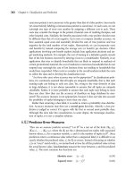
An information retrieval system often needs to trade off recall for precision or vice
versa. One commonly used trade-off is the F-score, which is defined as the harmonic
mean of recall and precision:
F
score =
recall × precision
(recall + precision)/2
.
The harmonic mean discourages a system that sacrifices one measure for another too
drastically.
All documents

Retrieved
documents
Relevant
documents
Relevant and
retrieved
Figure 10.6 Relationship between the set of relevant documents and the set of retrieved documents.
10.4 Text Mining 617
Precision, recall, and F-score are the basic measures of a retrieved set of documents.
These three measures are not directly useful for comparing two ranked listsof documents
because they are not sensitive to the internal ranking of the documents in a retrieved set.
In order to measure the quality of a ranked list of documents, it is common to compute an
average of precisions at all the ranks where a new relevant document is returned. It is also
common to plot a graph of precisions at many different levels of recall; a higher curve
represents a better-quality information retrieval system. For more details about these
measures, readers may consult an information retrieval textbook, such as [BYRN99].
Text Retrieval Methods
“What methods are there for information retrieval?” Broadly speaking, retrieval methods
fall into two categories: They generally either view the retrieval problem as a document
selection problem or as a document ranking problem.
In document selection methods, the query is regarded as specifying constraints for
selecting relevant documents. A typical method of this category is the Boolean retrieval
model, in which a document is represented by a set of keywords and a user provides
a Boolean expression of keywords, such as “car and repair shops,” “tea or coffee,” or
“database systems but not Oracle.” The retrieval system would take such a Boolean query
and return documents that satisfy the Boolean expression. Because of the difficulty in
prescribing a user’s information need exactly with a Boolean query, the Boolean retrieval
method generally only works well when the user knows a lot about the document collec-
tion and can formulate a good query in this way.
Document ranking methods use the query to rank all documents in the order of

relevance. For ordinary users and exploratory queries, these methods are more appro-
priate than document selection methods. Most modern information retrieval systems
present a ranked list of documents in response to a user’s keyword query. There are
many different ranking methods based on a large spectrum of mathematical founda-
tions, including algebra, logic, probability, and statistics. The common intuition behind
all of these methods is that we may match the keywords in a query with those in the
documents and score each document based on how well it matches the query. The goal
is to approximate the degree of relevance of a document with a score computed based on
information such as the frequency of words in the document and the whole collection.
Notice that it is inherently difficult to provide a precise measure of the degree of relevance
between a set of keywords. For example, it is difficult to quantify the distance between
data mining and data analysis. Comprehensive empirical evaluation is thus essential for
validating any retrieval method.
A detailed discussion of all of these retrieval methods is clearly out of the scope of this
book. Following we briefly discuss the most popular approach—the vector space model.
For other models, readers may refer to information retrieval textbooks, as referenced
in the bibliographic notes. Although we focus on the vector space model, some steps
discussed are not specific to this particular approach.
The basic idea of the vector space model is the following: We represent a document
and a query both as vectors in a high-dimensional space corresponding to all the
618 Chapter 10 Mining Object, Spatial, Multimedia, Text, and Web Data
keywords and use an appropriate similarity measure to compute the similarity between
the query vector and the document vector. The similarity values can then be used for
ranking documents.
“How do we tokenize text?” The first step in most retrieval systems is to identify key-
words for representing documents, a preprocessing step often called tokenization. To
avoid indexing useless words, a text retrieval system often associates a stop list with a set
of documents. A stop list is a set of words that are deemed “irrelevant.” For example, a,
the, of, for, with, and so on are stop words, even though they may appear frequently. Stop
lists may vary per document set. For example, database systems could be an important

keyword in a newspaper. However, it may be considered as a stop word in a set of research
papers presented in a database systems conference.
A group of different words may share the same word stem. A text retrieval system
needs to identify groups of words where the words in a group are small syntactic variants
of one another and collect only the common word stem per group. For example, the
group of words drug, drugged, and drugs, share a common word stem, drug, and can be
viewed as different occurrences of the same word.
“How can we model a document to facilitate information retrieval?” Starting with a set
of d documents and a set of t terms, we can model each document as a vector v in the
t dimensional space
t
, which is why this method is called the vector-space model. Let
the term frequency be the number of occurrences of term t in the document d, that is,
freq(d,t). The (weighted) term-frequency matrix TF(d,t) measures the association of a
term t with respect to the given document d: it is generally defined as 0 if the document
does not contain the term, and nonzero otherwise. There are many ways to define the
term-weighting for the nonzero entries in such a vector. For example, we can simply set
TF(d,t) = 1 if the term t occurs in the document d, or use the term frequency freq(d,t),
or the relative term frequency, that is, the term frequency versus the total number of
occurrences of all the terms in the document. There are also other ways to normalize the
term frequency. For example, the Cornell SMART system uses the following formula to
compute the (normalized) term frequency:
TF(d,t) =

0 if freq(d,t) = 0
1+ log(1 +log(freq(d,t))) otherwise.
(10.3)
Besides the term frequency measure, there is another important measure, called
inverse document frequency (IDF), that represents the scaling factor, or the importance,
of a term t. If a term t occurs in many documents, its importance will be scaled down

due to its reduced discriminative power. For example, the term database systems may
likely be less important if it occurs in many research papers in a database system confer-
ence. According to the same Cornell SMART system, IDF(t) is defined by the following
formula:
IDF(t) = log
1+ |d|
|d
t
|
, (10.4)
where d is the document collection, and d
t
is the set of documents containing term t. If
|d
t
| |d|, the term t will have a large IDF scaling factor and vice versa.
10.4 Text Mining 619
In a complete vector-space model, TF and IDF are combined together, which forms
the TF-IDF measure:
TF-IDF(d,t) = TF(d,t) ×IDF(t). (10.5)
Let us examine how to compute similarity among a set of documents based on the
notions of term frequency and inverse document frequency.
Example 10.9
Term frequency and inverse document frequency. Table 10.5 shows a term frequency
matrix where each row represents a document vector, each column represents a term,
and each entry registers freq(d
i
,t
j
), the number of occurrences of term t

j
in document d
i
.
Based on this table we can calculate the TF-IDF value of a term in a document. For
example, for t
6
in d
4
, we have
TF(d
4
,t
6
) = 1 +log(1+ log(15)) = 1.3377
IDF(t
6
) = log
1+ 5
3
= 0.301.
Therefore,
TF-IDF(d
4
,t
6
) = 1.3377 ×0.301 = 0.403
“How can we determine if two documents are similar?” Since similar documents are
expected to have similar relative term frequencies, we can measure the similarity among a
set of documents or between adocument and a query (often defined as a set of keywords),

based on similar relative term occurrences in the frequency table. Many metrics have
been proposed for measuring document similarity based on relative term occurrences
or document vectors. A representative metric is the cosine measure, defined as follows.
Let v
1
and v
2
be two document vectors. Their cosine similarity is defined as
sim(v
1
,v
2
) =
v
1
·v
2
|v
1
||v
2
|
, (10.6)
where the inner product v
1
·v
2
is the standard vector dot product, defined as Σ
t
i=1

v
1i
v
2i
,
and the norm |v
1
| in the denominator is defined as |v
1
| =
√
v
1
·v
1
.
Table 10.5 A term frequency matrix showing the frequency of terms per document.
document/term t
1
t
2
t
3
t
4
t
5
t
6
t

7
d
1
0 4 10 8 0 5 0
d
2
5 19 7 16 0 0 32
d
3
15 0 0 4 9 0 17
d
4
22 3 12 0 5 15 0
d
5
0 7 0 9 2 4 12
620 Chapter 10 Mining Object, Spatial, Multimedia, Text, and Web Data
Text Indexing Techniques
There are several popular text retrieval indexing techniques, including inverted indices
and signature files.
An inverted index is an index structure that maintains two hash indexed or B+-tree
indexed tables: document
table and term table, where
document table consists of a set of document records, each containing two fields:
doc id and posting list, where posting list is a list of terms (or pointers to terms) that
occur in the document, sorted according to some relevance measure.
term table consists of a set of term records, each containing two fields: term id and
posting
list, where posting list specifies a list of document identifiers in which the term
appears.

With such organization, it is easy to answer queries like “Find all of the documents asso-
ciated with a given set of terms,” or “Find all of the terms associated with a given set of
documents.” For example, to find all of the documents associated with a set of terms, we
can first find a list of document identifiers in term
table for each term, and then inter-
sect them to obtain the set of relevant documents. Inverted indices are widely used in
industry. They are easy to implement. The posting
lists could be rather long, making the
storage requirement quite large. They are easy to implement, but are not satisfactory at
handling synonymy (where two very different words can have the same meaning) and
polysemy (where an individual word may have many meanings).
A signature file is a file that stores a signature record for each document in the database.
Each signature has a fixed size of b bits representing terms. A simple encoding scheme
goes as follows. Each bit of a document signature is initialized to 0. A bit is set to 1 if the
term it represents appears in the document. A signature S
1
matches another signature S
2
if each bit that is set in signature S
2
is also set in S
1
. Since there are usually more terms
than available bits, multiple terms may be mapped into the same bit. Such multiple-to-
one mappings make the search expensive because a document that matches the signature
of a query does not necessarily contain the set of keywords of the query. The document
has to be retrieved, parsed, stemmed, and checked. Improvements can be made by first
performing frequency analysis, stemming, and by filtering stop words, and then using a
hashing technique and superimposed coding technique to encode the list of terms into
bit representation. Nevertheless, the problem of multiple-to-one mappings still exists,

which is the major disadvantage of this approach.
Readers can refer to [WMB99] for more detailed discussion of indexing techniques,
including how to compress an index.
Query Processing Techniques
Once an inverted index is created for a document collection, a retrieval system can answer
a keyword query quickly by looking up which documents contain the query keywords.
Specifically, we will maintain a score accumulator for each document and update these