Database systems concepts 4th edition phần 10 pptx

Silberschatz−Korth−Sudarshan:

Database System
Concepts, Fourth Edition
VII. Other Topics 22. Advanced Querying and
Information Retrieval
825
© The McGraw−Hill
Companies, 2001
832 Chapter 22 Advanced Querying and Information Retrieval
22.3.2 Classification
As mentioned in Section 22.3.1, prediction is one of the most important types of data
mining. We outline what is classification, study techniques for building one type of
classifiers, called decision tree classifiers, and then study other prediction techniques.
Abstractly, the classification problem is this: Given that items belong to one of
several classes, and given past instances (called training instances)ofitemsalong
with the classes to which they belong, the problem is to predict the class to which a
new item belongs. The class of the new instance is not known, so other attributes of
theinstancemustbeusedtopredicttheclass.
Classification can be done by finding rules that partition the given data into
disjoint groups. For instance, suppose that a credit-card company wants to decide
whether or not to give a credit card to an applicant. The company has a variety of
information about the person, such as her age, educational background, annual in-
come, and current debts, that it can use for making a decision.
Some of this information could be relevant to the credit worthiness of the appli-
cant, whereas some may not be. To make the decision, the company assigns a credit-
worthiness level of excellent, good, average, or bad to each of a sample set of cur-
rent customers according to each customer’s payment history. Then, the company
attempts to find rules that classify its current customers into excellent, good, aver-
age, or bad, on the basis of the information about the person, other than the actual
payment history (which is unavailable for new customers). Let us consider just two

attributes: education level (highest degree earned) and income. The rules may be of
the following form:
∀person P, P .degree = masters and P.income > 75, 000
⇒ P.credit = excellent
∀ person P, P .degree = bachelors or
(P.income ≥ 25, 000 and P .income ≤ 75, 000) ⇒ P.credit = good
Similar rules would also be present for the other credit worthiness levels (average
and bad).
The process of building a classifier starts from a sample of data, called a training
set. For each tuple in the training set, the class to which the tuple belongs is already
known. For instance, the training set for a credit-card application may be the existing
customers, with their credit worthiness determined from their payment history. The
actual data, or population, may consist of all people, including those who are not
existing customers. There are several ways of building a classifier, as we shall see.
22.3.2.1 Decision Tree Classifiers
The decision tree classifier is a widely used technique for classification. As the name
suggests, decision tree classifiers use a tree; each leaf node has an associated class,
and each internal node has a predicate (or more generally, a function) associated with
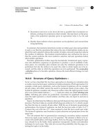
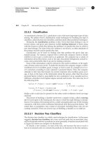
it. Figure 22.6 shows an example of a decision tree.
To classify a new instance, we start at the root, and traverse the tree to reach a
leaf; at an internal node we evaluate the predicate (or function) on the data instance,
Silberschatz−Korth−Sudarshan:

Database System
Concepts, Fourth Edition
VII. Other Topics 22. Advanced Querying and
Information Retrieval
826
© The McGraw−Hill
Companies, 2001

22.3 Data Mining 833
degree
income
income
income
income
bachelors
masters
doctorate
none
bad
average
good
bad
average
good
excellent
<50K
>100K
<25K >=25K
>=50K
<50K
<25K
>75K
25 to 75K
50 to 100K
Figure 22.6 Classification tree.
to find which child to go to. The process continues till we reach a leaf node. For
example, if the degree level of a person is masters, and the persons income is 40K,
starting from the root we follow the edge labeled “masters,” and from there the edge

labeled “25K to 75K,” to reach a leaf. The class at the leaf is “good,” so we predict that
thecreditriskofthatpersonisgood.
Building Decision Tree Classifiers
The question then is how to build a decision tree classifier, given a set of training
instances. The most common way of doing so is to use a greedy algorithm, which
works recursively, starting at the root and building the tree downward. Initially there
is only one node, the root, and all training instances are associated with that node.
At each node, if all, or “almost all” training instances associated with the node be-
long to the same class, then the node becomes a leaf node associated with that class.
Otherwise, a partitioning attribute and partitioning conditions must be selected to
create child nodes. The data associated with each child node is the set of training
instances that satisfy the partitioning condition for that child node. In our example,
the attribute degree is chosen, and four children, one for each value of degree, are cre-
ated. The conditions for the four children nodes are degree =none,degree =bachelors,
degree =masters,anddegree = doctorate, respectively. The data associated with each
child consist of training instances satisfying the condition associated with that child.
At the node corresponding to masters, the attribute income is chosen, with the range
of values partitioned into intervals 0 to 25,000, 25,000 to 50,000, 50,000 to 75,000, and
over 75,000. The data associated with each node consist of training instances with the
degree attribute being masters, and the income attribute being in each of these ranges,
Silberschatz−Korth−Sudarshan:

Database System
Concepts, Fourth Edition
VII. Other Topics 22. Advanced Querying and
Information Retrieval
827
© The McGraw−Hill
Companies, 2001
834 Chapter 22 Advanced Querying and Information Retrieval

respectively. As an optimization, since the class for the range 25,000 to 50,000 and the
range 50,000 to 75,000 is the same under the node degree = masters, the two ranges
have been merged into a single range 25,000 to 75,000.
Best Splits
Intuitively, by choosing a sequence of partitioning attributes, we start with the set
of all training instances, which is “impure” in the sense that it contains instances
from many classes, and end up with leaves which are “pure” in the sense that at
each leaf all training instances belong to only one class. We shall see shortly how to
measure purity quantitatively. To judge the benefit of picking a particular attribute
and condition for partitioning of the data at a node, we measure the purity of the
data at the children resulting from partitioning by that attribute. The attribute and
condition that result in the maximum purity are chosen.
The purity of a set S of training instances can be measured quantitatively in several
ways. Suppose there are k classes, and of the instances in S the fraction of instances
in class i is p
i
. One measure of purity, the Gini measure is defined as
Gini(S)=1−
k

i−1
p
2
i
When all instances are in a single class, the Gini value is 0, while it reaches its max-
imum (of 1 −1/k) if each class has the same number of instances. Another measure
of purity is the entropy measure, which is defined as
Entropy(S)=−
k


i−1
p
i
log
2
p
i
The entropy value is 0 if all instances are in a single class, and reaches its maximum
when each class has the same number of instances. The entropy measure derives
from information theory.
When a set S is split into multiple sets S
i
,i=1, 2, ,r, we can measure the purity
of the resultant set of sets as:
Purity(S
1
,S
2
, ,S
r
)=
r

i=1
|S
i
|
|S|
purity(S
i

)
That is, the purity is the weighted average of the purity of the sets S
i
.Theabove
formula can be used with both the Gini measure and the entropy measure of purity.
The information gain due to a particular split of S into S
i
,i=1, 2, ,ris then
Information-gain(S, {S
1
,S
2
, ,S
r
}) = purity(S) − purity(S
1
,S
2
, ,S
r
)
Splits into fewer sets are preferable to splits into many sets, since they lead to
simpler and more meaningful decision trees. The number of elements in each of the
sets S
i
may also be taken into account; otherwise, whether a set S
i
has 0 elements or
1 element would make a big difference in the number of sets, although the split is the
same for almost all the elements. The information content of a particular split can be

Silberschatz−Korth−Sudarshan:

Database System
Concepts, Fourth Edition
VII. Other Topics 22. Advanced Querying and
Information Retrieval
828
© The McGraw−Hill
Companies, 2001
22.3 Data Mining 835
defined in terms of entropy as
Information-content(S, {S
1
,S
2
, ,S
r
})) = −
r

i−1
|S
i
|
|S|
log
2
|S
i
|

|S|
All of this leads to a definition: The best split for an attribute is the one that gives
the maximum information gain ratio, defined as
Information-gain(S, {S
1
,S
2
, ,S
r
})
Information-content(S, {S
1
,S
2
, ,S
r
})
Finding Best Splits
How do we find the best split for an attribute? How to split an attribute depends
on the type of the attribute. Attributes can be either continuous valued,thatis,the
values can be ordered in a fashion meaningful to classification, such as age or income,
or can be categorical, that is, they have no meaningful order, such as department
names or country names. We do not expect the sort order of department names or
country names to have any significance to classification.
Usually attributes that are numbers (integers/reals) are treated as continuous val-
ued while character string attributes are treated as categorical, but this may be con-
trolled by the user of the system. In our example, we have treated the attribute degree
as categorical, and the attribute income as continuous valued.
We first consider how to find best splits for continuous-valued attributes. For sim-
plicity, we shall only consider binary splits of continuous-valued attributes, that is,

splits that result in two children. The case of multiway splits is more complicated;
see the bibliographical notes for references on the subject.
To find the best binary split of a continuous-valued attribute, we first sort the at-
tribute values in the training instances. We then compute the information gain ob-
tained by splitting at each value. For example, if the training instances have values
1, 10, 15,and25 for an attribute, the split points considered are 1, 10,and15;ineach
case values less than or equal to the split point form one partition and the rest of the
values form the other partition. The best binary split for the attribute is the split that
gives the maximum information gain.
For a categorical attribute, we can have a multiway split, with a child for each
value of the attribute. This works fine for categorical attributes with only a few dis-
tinct values, such as degree or gender. However, if the attribute has many distinct
values, such as department names in a large company, creating a child for each value
is not a good idea. In such cases, we would try to combine multiple values into each
child, to create a smaller number of children. See the bibliographical notes for refer-
ences on how to do so.
Decision-Tree Construction Algorithm
The main idea of decision tree construction is to evaluate different attributes and dif-
ferent partitioning conditions, and pick the attribute and partitioning condition that
results in the maximum information gain ratio. The same procedure works recur-
Silberschatz−Korth−Sudarshan:

Database System
Concepts, Fourth Edition
VII. Other Topics 22. Advanced Querying and
Information Retrieval
829
© The McGraw−Hill
Companies, 2001
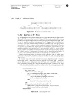
836 Chapter 22 Advanced Querying and Information Retrieval

procedure GrowTree(S)
Partition(S);
procedure Partition (S)
if (purity(S) >δ
p
or |S| <δ
s
) then
return;
for each attribute A
evaluate splits on attribute A;
Use best split found (across all attributes) to partition
S into S
1
,S
2
, ,S
r
;
for i =1, 2, ,r
Partition(S
i
);
Figure 22.7 Recursive construction of a decision tree.
sively on each of the sets resulting from the split, thereby recursively constructing
a decision tree. If the data can be perfectly classified, the recursion stops when the
purity of a set is 0. However, often data are noisy, or a set may be so small that par-
titioning it further may not be justified statistically. In this case, the recursion stops
when the purity of a set is “sufficiently high,” and the class of resulting leaf is defined
as the class of the majority of the elements of the set. In general, different branches of

the tree could grow to different levels.
Figure 22.7 shows pseudocode for a recursive tree construction procedure, which
takes a set of training instances S as parameter. The recursion stops when the set is
sufficiently pure or the set S is too small for further partitioning to be statistically
significant. The parameters δ
p
and δ
s
define cutoffs for purity and size; the system
may give them default values, that may be overridden by users.
There are a wide variety of decision tree construction algorithms, and we outline
the distinguishing features of a few of them. See the bibliographical notes for details.
With very large data sets, partitioning may be expensive, since it involves repeated
copying. Several algorithms have therefore been developed to minimize the
I/O and
computation cost when the training data are larger than available memory.
Several of the algorithms also prune subtrees of the generated decision tree to
reduce overfitting: A subtree is overfitted if it has been so highly tuned to the specifics
of the training data that it makes many classification errors on other data. A subtree
is pruned by replacing it with a leaf node. There are different pruning heuristics;
one heuristic uses part of the training data to build the tree and another part of the
training data to test it. The heuristic prunes a subtree if it finds that misclassification
on the test instances would be reduced if the subtree were replaced by a leaf node.
We can generate classification rules from a decision tree, if we so desire. For each
leaf we generate a rule as follows: The left-hand side is the conjunction of all the split
conditions on the path to the leaf, and the class is the class of the majority of the
training instances at the leaf. An example of such a classification rule is
degree = masters and income > 75, 000 ⇒ excellent
Silberschatz−Korth−Sudarshan:

Database System
Concepts, Fourth Edition
VII. Other Topics 22. Advanced Querying and
Information Retrieval
830
© The McGraw−Hill
Companies, 2001
22.3 Data Mining 837
22.3.2.2 Other Types of Classifiers
There are several types of classifiers other than decision tree classifiers. Two types
that have been quite useful are neural net classifiers and Bayesian classifiers. Neural net
classifiers use the training data to train artificial neural nets. There is a large body of
literature on neural nets, and we do not consider them further here.
Bayesian classifiers find the distribution of attribute values for each class in the
training data; when given a new instance d, they use the distribution information to
estimate, for each class c
j
, the probability that instance d belongs to class c
j
, denoted
by p(c
j
|d), in a manner outlined here. The class with maximum probability becomes
the predicted class for instance d.
To find the probability p(c
j
|d) of instance d being in class c
j
, Bayesian classifiers
use Bayes’ theorem,whichsays

p(c
j
|d)=
p(d|c
j
)p(c
j
)
p(d)
where p(d|c
j
) is the probability of generating instance d given class c
j
, p(c
j
) is the
probability of occurrence of class c
j
,andp(d) is the probability of instance d occur-
ring. Of these, p(d) can be ignored since it is the same for all classes. p(c
j
) is simply
the fraction of training instances that belong to class c
j
.
Finding p(d|c
j
) exactly is difficult, since it requires a complete distribution of in-
stances of c
j

. To simplify the task, naive Bayesian classifiers assume attributes have
independent distributions, and thereby estimate
p(d|c
j
)=p(d
1
|c
j
) ∗ p(d
2
|c
j
) ∗ ∗ p(d
n
|c
j
)
That is, the probability of the instance d occurring is the product of the probability of
occurrence of each of the attribute values d
i
of d, given the class is c
j
.
The probabilities p(d
i
|c
j
) derive from the distribution of values for each attribute i,
for each class class c
j

. This distribution is computed from the training instances that
belong to each class c
j
; the distribution is usually approximated by a histogram. For
instance, we may divide the range of values of attribute i into equal intervals, and
store the fraction of instances of class c
j
that fall in each interval. Given a value d
i
for
attribute i,thevalueofp(d
i
|c
j
) is simply the fraction of instances belonging to class
c
j
that fall in the interval to which d
i
belongs.
A significant benefit of Bayesian classifiers is that they can classify instances with
unknown and null attribute values—unknown or null attributes are just omitted
from the probability computation. In contrast, decision tree classifiers cannot mean-
ingfully handle situations where an instance to be classified has a null value for a
partitioning attribute used to traverse further down the decision tree.
22.3.2.3 Regression
Regression deals with the prediction of a value, rather than a class. Given values for
asetofvariables,X
1
,X

2
, ,X
n
, we wish to predict the value of a variable Y .For
instance, we could treat the level of education as a number and income as another
number, and, on the basis of these two variables, we wish to predict the likelihood of
Silberschatz−Korth−Sudarshan:

Database System
Concepts, Fourth Edition
VII. Other Topics 22. Advanced Querying and
Information Retrieval
831
© The McGraw−Hill
Companies, 2001
838 Chapter 22 Advanced Querying and Information Retrieval
default, which could be a percentage chance of defaulting, or the amount involved in
the default.
One way is to infer coefficients a
0
,a
1
,a
1
, ,a
n
such that
Y = a
0
+ a

1
∗ X
1
+ a
2
∗ X
2
+ ···+ a
n
∗ X
n
Finding such a linear polynomial is called linear regression. In general, we wish to
find a curve (defined by a polynomial or other formula) that fits the data; the process
is also called curve fitting.
The fit may only be approximate, because of noise in the data or because the rela-
tionship is not exactly a polynomial, so regression aims to find coefficients that give
the best possible fit. There are standard techniques in statistics for finding regression
coefficients. We do not discuss these techniques here, but the bibliographical notes
provide references.
22.3.3 Association Rules
Retail shops are often interested in associations between different items that people
buy. Examples of such associations are:
• Someone who buys bread is quite likely also to buy milk
• A person who bought the book Database System Concepts is quite likely also to
buy the book Operating System Concepts.
Association information can be used in several ways. When a customer buys a partic-
ular book, an online shop may suggest associated books. A grocery shop may decide
to place bread close to milk, since they are often bought together, to help shoppers fin-
ish their task faster. Or the shop may place them at opposite ends of a row, and place
other associated items in between to tempt people to buy those items as well, as the

shoppers walk from one end of the row to the other. A shop that offers discounts on
one associated item may not offer a discount on the other, since the customer will
probably buy the other anyway.
Association Rules
An example of an association rule is
bread ⇒ milk
In the context of grocery-store purchases, the rule says that customers who buy bread
also tend to buy milk with a high probability. An association rule must have an asso-
ciated population: the population consists of a set of instances. In the grocery-store
example, the population may consist of all grocery store purchases; each purchase is
an instance. In the case of a bookstore, the population may consist of all people who
made purchases, regardless of when they made a purchase. Each customer is an in-
stance. Here, the analyst has decided that when a purchase is made is not significant,
whereas for the grocery-store example, the analyst may have decided to concentrate
on single purchases, ignoring multiple visits by the same customer.
Silberschatz−Korth−Sudarshan:

Database System
Concepts, Fourth Edition
VII. Other Topics 22. Advanced Querying and
Information Retrieval
832
© The McGraw−Hill
Companies, 2001
22.3 Data Mining 839
Rules have an associated support,aswellasanassociatedconfidence.Theseare
defined in the context of the population:
• Support is a measure of what fraction of the population satisfies both the an-
tecedent and the consequent of the rule.
For instance, suppose only 0.001 percent of all purchases include milk and

screwdrivers. The support for the rule
milk ⇒ screwdrivers
is low. The rule may not even be statistically significant—perhaps there was
only a single purchase that included both milk and screwdrivers. Businesses
are usually not interested in rules that have low support, since they involve
few customers, and are not worth bothering about.
On the other hand, if 50 percent of all purchases involve milk and bread,
then support for rules involving bread and milk (and no other item) is rela-
tively high, and such rules may be worth attention. Exactly what minimum
degree of support is considered desirable depends on the application.
• Confidence is a measure of how often the consequent is true when the an-
tecedent is true. For instance, the rule
bread ⇒ milk
has a confidence of 80 percent if 80 percent of the purchases that include bread
also include milk. A rule with a low confidence is not meaningful. In busi-
ness applications, rules usually have confidences significantly less than 100
percent, whereas in other domains, such as in physics, rules may have high
confidences.
Note that the confidence of bread ⇒ milk maybeverydifferentfromthe
confidence of milk ⇒ bread, although both have the same support.
Finding Association Rules
To discover association rules of the form
i
1
,i
2
, ,i
n
⇒ i
0

we first find sets of items with sufficient support, called large itemsets.Inourexam-
ple we find sets of items that are included in a sufficiently large number of instances.
We will shortly see how to compute large itemsets.
For each large itemset, we then output all rules with sufficient confidence that
involve all and only the elements of the set. For each large itemset S,weoutputa
rule S − s ⇒ s for every subset s ⊂ S,providedS − s ⇒ s has sufficient confidence;
the confidence of the rule is given by support of s divided by support of S.
We now consider how to generate all large itemsets. If the number of possible sets
of items is small, a single pass over the data suffices to detect the level of support
for all the sets. A count, initialized to 0, is maintained for each set of items. When a
purchase record is fetched, the count is incremented for each set of items such that
Silberschatz−Korth−Sudarshan:

Database System
Concepts, Fourth Edition
VII. Other Topics 22. Advanced Querying and
Information Retrieval
833
© The McGraw−Hill
Companies, 2001
840 Chapter 22 Advanced Querying and Information Retrieval
all items in the set are contained in the purchase. For instance, if a purchase included
items a, b,andc, counts would be incremented for {a}, {b}, {c}, {a, b}, {b, c}, {a, c},
and {a, b, c}. Those sets with a sufficiently high count at the end of the pass corre-
spond to items that have a high degree of association.
The number of sets grows exponentially, making the procedure just described in-
feasible if the number of items is large. Luckily, almost all the sets would normally
have very low support; optimizations have been developed to eliminate most such
sets from consideration. These techniques use multiple passes on the database, con-
sidering only some sets in each pass.

In the aprioritechnique for generating large itemsets, only sets with single items
are considered in the first pass. In the second pass, sets with two items are considered,
and so on.
At the end of a pass all sets with sufficient support are output as large itemsets.
Sets found to have too little support at the end of a pass are eliminated. Once a set is
eliminated, none of its supersets needs to be considered. In other words, in pass i we
need to count only supports for sets of size i such that all subsets of the set have been
found to have sufficiently high support; it suffices to test all subsets of size i − 1 to
ensure this property. At the end of some pass i, we would find that no set of size i has
sufficient support, so we do not need to consider any set of size i +1. Computation
then terminates.
22.3.4 Other Types of Associations
Using plain association rules has several shortcomings. One of the major shortcom-
ings is that many associations are not very interesting, since they can be predicted.
For instance, if many people buy cereal and many people buy bread, we can predict
that a fairly large number of people would buy both, even if there is no connection be-
tween the two purchases. What would be interesting is a deviation from the expected
co-occurrence of the two. In statistical terms, we look for correlations between items;
correlations can be positive, in that the co-occurrence is higher than would have been
expected, or negative, in that the items co-occur less frequently than predicted. See a
standard textbook on statistics for more information about correlations.
Another important class of data-mining applications is sequence associations (or
correlations). Time-series data, such as stock prices on a sequence of days, form an
example of sequence data. Stock-market analysts want to find associations among
stock-market price sequences. An example of such a association is the following rule:
“Whenever bond rates go up, the stock prices go down within 2 days.” Discover-
ing such association between sequences can help us to make intelligent investment
decisions. See the bibliographical notes for references to research on this topic.
Deviations from temporal patterns are often interesting. For instance, if a company
has been growing at a steady rate each year, a deviation from the usual growth rate

is surprising. If sales of winter clothes go down in summer, it is not surprising, since
we can predict it from past years; a deviation that we could not have predicted from
past experience would be considered interesting. Mining techniques can find devia-
tions from what one would have expected on the basis of past temporal/sequential
patterns. See the bibliographical notes for references to research on this topic.
Silberschatz−Korth−Sudarshan:

Database System
Concepts, Fourth Edition
VII. Other Topics 22. Advanced Querying and
Information Retrieval
834
© The McGraw−Hill
Companies, 2001
22.3 Data Mining 841
22.3.5 Clustering
Intuitively, clustering refers to the problem of finding clusters of points in the given
data. The problem of clustering can be formalized from distance metrics in several
ways. One way is to phrase it as the problem of grouping points into k sets (for a
given k) so that the average distance of points from the centroid of their assigned
cluster is minimized.
5
Another way is to group points so that the average distance
between every pair of points in each cluster is minimized. There are other defini-
tions too; see the bibliographical notes for details. But the intuition behind all these
definitions is to group similar points together in a single set.
Another type of clustering appears in classification systems in biology. (Such clas-
sification systems do not attempt to predict classes, rather they attempt to cluster re-
lated items together.) For instance, leopards and humans are clustered under the class
mammalia, while crocodiles and snakes are clustered under reptilia. Both mammalia

and reptilia come under the common class chordata. The clustering of mammalia has
further subclusters, such as carnivora and primates. We thus have hierarchical clus-
tering. Given characteristics of different species, biologists have created a complex
hierarchical clustering scheme grouping related species together at different levels of
the hierarchy.
Hierarchical clustering is also useful in other domains—for clustering documents,
for example. Internet directory systems (such as Yahoo’s) cluster related documents
in a hierarchical fashion (see Section 22.5.5). Hierarchical clustering algorithms can
be classified as agglomerative clustering algorithms, which start by building small
clusters and then creater higher levels, or divisive clustering algorithms, which first
create higher levels of the hierarchical clustering, then refine each resulting cluster
into lower level clusters.
The statistics community has studied clustering extensively. Database research has
provided scalable clustering algorithms that can cluster very large data sets (that may
not fit in memory). The Birch clustering algorithm is one such algorithm. Intuitively,
data points are inserted into a multidimensional tree structure (based on R-trees, de-
scribed in Section 23.3.5.3), and guided to appropriate leaf nodes based on nearness
to representative points in the internal nodes of the tree. Nearby points are thus clus-
tered together in leaf nodes, and summarized if there are more points than fit in
memory. Some postprocessing after insertion of all points gives the desired overall
clustering. See the bibliographical notes for references to the Birch algorithm, and
other techniques for clustering, including algorithms for hierarchical clustering.
An interesting application of clustering is to predict what new movies (or books,
or music) a person is likely to be interested in, on the basis of:
1. The person’s past preferences in movies
2. Other people with similar past preferences
3. The preferences of such people for new movies
5. The centroid of a set of points is defined as a point whose coordinate on each dimension is the average
of the coordinates of all the points of that set on that dimension. For example in two dimensions, the
centroid of a set of points { (x

1
,y
1
), (x
2
,y
2
), ,(x
n
,y
n
) } is given by (
n
i=1
x
i
n
,
n
i=1
y
i
n
)
Silberschatz−Korth−Sudarshan:

Database System
Concepts, Fourth Edition
VII. Other Topics 22. Advanced Querying and
Information Retrieval

835
© The McGraw−Hill
Companies, 2001
842 Chapter 22 Advanced Querying and Information Retrieval
One approach to this problem is as follows. To find people with similar past prefer-
ences we create clusters of people based on their preferences for movies. The accuracy
of clustering can be improved by previously clustering movies by their similarity, so
even if people have not seen the same movies, if they have seen similar movies they
would be clustered together. We can repeat the clustering, alternately clustering peo-
ple, then movies, then people, and so on till we reache an equilibrium. Given a new
user, we find a cluster of users most similar to that user, on the basis of the user’s
preferences for movies already seen. We then predict movies in movie clusters that
are popular with that user’s cluster as likely to be interesting to the new user. In fact,
this problem is an instance of collaborative filtering, where users collaborate in the task
of filtering information to find information of interest.
22.3.6 Other Types of Mining
Text mining applies data mining techniques to textual documents. For instance, there
are tools that form clusters on pages that a user has visited; this helps users when
they browse the history of their browsing to find pages they have visited earlier. The
distance between pages can be based, for instance, on common words in the pages
(see Section 22.5.1.3). Another application is to classify pages into a Web directory
automatically, according to their similarity with other pages (see Section 22.5.5).
Data-visualization systems help users to examine large volumes of data, and to
detect patterns visually. Visual displays of data—such as maps, charts, and other
graphical representations—allow data to be presented compactly to users. A sin-
gle graphical screen can encode as much information as a far larger number of text
screens. For example, if the user wants to find out whether production problems at
plants are correlated to the locations of the plants, the problem locations can be en-
coded in a special color—say, red—on a map. The user can then quickly discover
locations where problems are occurring. The user may then form hypotheses about

why problems are occurring in those locations, and may verify the hypotheses quan-
titatively against the database.
As another example, information about values can be encoded as a color, and can
be displayed with as little as one pixel of screen area. To detect associations between
pairs of items, we can use a two-dimensional pixel matrix, with each row and each
column representing an item. The percentage of transactions that buy both items can
be encoded by the color intensity of the pixel. Items with high association will show
up as bright pixels in the screen—easy to detect against the darker background.
Data visualization systems do not automatically detect patterns, but provide sys-
tem support for users to detect patterns. Since humans are very good at detecting
visual patterns, data visualization is an important component of data mining.
22.4 Data Warehousing
Large companies have presences in many places, each of which may generate a large
volume of data. For instance, large retail chains have hundreds or thousands of stores,
whereas insurance companies may have data from thousands of local branches. Fur-
ther, large organizations have a complex internal organization structure, and there-
Silberschatz−Korth−Sudarshan:

Database System
Concepts, Fourth Edition
VII. Other Topics 22. Advanced Querying and
Information Retrieval
836
© The McGraw−Hill
Companies, 2001
22.4 Data Warehousing 843
data
loaders
DBMS
data warehouse

query and
analysis tools
data source n
data source 2
data source 1
…
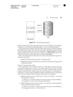
Figure 22.8 Data-warehouse architecture.
fore different data may be present in different locations, or on different operational
systems, or under different schemas. For instance, manufacturing-problem data and
customer-complaint data may be stored on different database systems. Corporate de-
cision makers require access to information from all such sources. Setting up queries
on individual sources is both cumbersome and inefficient. Moreover, the sources of
data may store only current data, whereas decision makers may need access to past
data as well; for instance, information about how purchase patterns have changed in
the past year could be of great importance. Data warehouses provide a solution to
these problems.
A data warehouse is a repository (or archive) of information gathered from mul-
tiple sources, stored under a unified schema, at a single site. Once gathered, the data
are stored for a long time, permitting access to historical data. Thus, data warehouses
provide the user a single consolidated interface to data, making decision-support
queries easier to write. Moreover, by accessing information for decision support from
a data warehouse, the decision maker ensures that online transaction-processing sys-
tems are not affected by the decision-support workload.
22.4.1 Components of a Data Warehouse
Figure 22.8 shows the architecture of a typical data warehouse, and illustrates the
gathering of data, the storage of data, and the querying and data-analysis support.
Among the issues to be addressed in building a warehouse are the following:
• When and how to gather data. In a source-driven architecture for gather-
ing data, the data sources transmit new information, either continually (as
transaction processing takes place), or periodically (nightly, for example). In

a destination-driven architecture, the data warehouse periodically sends re-
quests for new data to the sources.
Silberschatz−Korth−Sudarshan:

Database System
Concepts, Fourth Edition
VII. Other Topics 22. Advanced Querying and
Information Retrieval
837
© The McGraw−Hill
Companies, 2001
844 Chapter 22 Advanced Querying and Information Retrieval
Unless updates at the sources are replicated at the warehouse via two-phase
commit, the warehouse will never be quite up to date with the sources. Two-
phase commit is usually far too expensive to be an option, so data warehouses
typically have slightly out-of-date data. That, however, is usually not a prob-
lem for decision-support systems.
• What schema to use. Data sources that have been constructed independently
are likely to have different schemas. In fact, they may even use different data
models. Part of the task of a warehouse is to perform schema integration, and
to convert data to the integrated schema before they are stored. As a result, the
data stored in the warehouse are not just a copy of the data at the sources. In-
stead, they can be thought of as a materialized view of the data at the sources.
• Data cleansing. The task of correcting and preprocessing data is called data
cleansing. Data sources often deliver data with numerous minor inconsisten-
cies, that can be corrected. For example, names are often misspelled, and ad-
dresses may have street/area/city names misspelled, or zip codes entered in-
correctly. These can be corrected to a reasonable extent by consulting a data-
base of street names and zip codes in each city. Address lists collected from
multiple sources may have duplicates that need to be eliminated in a merge–

purge operation. Records for multiple individuals in a house may be grouped
together so only one mailing is sent to each house; this operation is called
householding.
• How to propagate updates. Updates on relations at the data sources must
be propagated to the data warehouse. If the relations at the data warehouse
are exactly the same as those at the data source, the propagation is straight-
forward. If they are not, the problem of propagating updates is basically the
view-maintenance problem, which was discussed in Section 14.5.
• What data to summarize. The raw data generated by a transaction-processing
system may be too large to store online. However, we can answer many queries
by maintaining just summary data obtained by aggregation on a relation,
rather than maintaining the entire relation. For example, instead of storing
data about every sale of clothing, we can store total sales of clothing by item-
name and category.
Suppose that a relation r has been replaced by a summary relation s.Users
may still be permitted to pose queries as though the relation r were available
online. If the query requires only summary data, it may be possible to trans-
form it into an equivalent one using s instead; see Section 14.5.
22.4.2 Warehouse Schemas
Data warehouses typically have schemas that are designed for data analysis, using
tools such as
OLAP tools. Thus, the data are usually multidimensional data, with di-
mension attributes and measure attributes. Tables containing multidimensional data
are called fact tables and are usually very large. A table recording sales information
Silberschatz−Korth−Sudarshan:

Database System
Concepts, Fourth Edition
VII. Other Topics 22. Advanced Querying and
Information Retrieval

838
© The McGraw−Hill
Companies, 2001
22.4 Data Warehousing 845
for a retail store, with one tuple for each item that is sold, is a typical example of a fact
table. The dimensions of the sales table would include what the item is (usually an
item identifier such as that used in bar codes), the date when the item is sold, which
location (store) the item was sold from, which customer bought the item, and so on.
The measure attributes may include the number of items sold and the price of the
items.
To minimize storage requirements, dimension attributes are usually short identi-
fiers that are foreign keys into other other tables called dimension tables.For
instance, a fact table sales would have attributes item-id, store-id, customer-id,anddate,
and measure attributes number and price. The attribute store-id is a foreign key into
adimensiontablestore, which has other attributes such as store location (city, state,
country). The item-id attribute of the sales table would be a foreign key into a di-
mension table item-info, which would contain information such as the name of the
item, the category to which the item belongs, and other item details such as color and
size. The customer-id attribute would be a foreign key into a customer table containing
attributes such as name and address of the customer. We can also view the date at-
tribute as a foreign key into a date-info table giving the month, quarter, and year of
each date.
The resultant schema appears in Figure 22.9. Such a schema, with a fact table,
multiple dimension tables, and foreign keys from the fact table to the dimension ta-
bles, is called a star schema. More complex data warehouse designs may have multi-
ple levels of dimension tables; for instance, the item-info table may have an attribute
manufacturer-id that is a foreign key into another table giving details of the manufac-
turer. Such schemas are called snowflake schemas. Complex data warehouse designs
may also have more than one fact table.
item-id

store-id
store-id
item-id
itemname
color
size
item-info
sales
store
city
state
country
date
month
quarter
year
date-info
number
date
customer-id
customer
customer-id
name
street
city
state
zipcode
country
category
price

Figure 22.9 Star schema for a data warehouse.
Silberschatz−Korth−Sudarshan:

Database System
Concepts, Fourth Edition
VII. Other Topics 22. Advanced Querying and
Information Retrieval
839
© The McGraw−Hill
Companies, 2001
846 Chapter 22 Advanced Querying and Information Retrieval
22.5 Information-Retrieval Systems
The field of information retrieval has developed in parallel with the field of databases.
In the traditional model used in the field of information retrieval, information is orga-
nized into documents, and it is assumed that there is a large number of documents.
Data contained in documents is unstructured, without any associated schema. The
process of information retrieval consists of locating relevant documents, on the basis
of user input, such as keywords or example documents.
The Web provides a convenient way to get to, and to interact with, information
sources across the Internet. However, a persistent problem facing the Web is the ex-
plosion of stored information, with little guidance to help the user to locate what
is interesting. Information retrieval has played a critical role in making the Web a
productive and useful tool, especially for researchers.
Traditional examples of information-retrieval systems are online library catalogs
and online document-management systems such as those that store newspaper arti-
cles. The data in such systems are organized as a collection of documents; a newspaper
article or a catalog entry (in a library catalog) are examples of documents. In the con-
text of the Web, usually each
HTML page is considered to be a document.
A user of such a system may want to retrieve a particular document or a particular

class of documents. The intended documents are typically described by a set of key-
words—for example, the keywords “database system” may be used to locate books
on database systems, and the keywords “stock” and “scandal” may be used to locate
articles about stock-market scandals. Documents have associated with them a set of
keywords, and documents whose keywords contain those supplied by the user are
retrieved.
Keyword-based information retrieval can be used not only for retrieving textual
data, but also for retrieving other types of data, such as video or audio data, that
have descriptive keywords associated with them. For instance, a video movie may
have associated with it keywords such as its title, director, actors, type, and so on.
There are several differences between this model and the models used in tradi-
tional database systems.
• Database systems deal with several operations that are not addressed in infor-
mation-retrieval systems. For instance, database systems deal with updates
and with the associated transactional requirements of concurrency control
and durability. These matters are viewed as less important in information sys-
tems. Similarly, database systems deal with structured information organized
with relatively complex data models (such as the relational model or object-
oriented data models), whereas information-retrieval systems traditionally
have used a much simpler model, where the information in the database is
organized simply as a collection of unstructured documents.
• Information-retrieval systems deal with several issues that have not been ad-
dressed adequately in database systems. For instance, the field of information
retrieval has dealt with the problems of managing unstructured documents,
such as approximate searching by keywords, and of ranking of documents on
estimated degree of relevance of the documents to the query.
Silberschatz−Korth−Sudarshan:

Database System
Concepts, Fourth Edition

VII. Other Topics 22. Advanced Querying and
Information Retrieval
840
© The McGraw−Hill
Companies, 2001
22.5 Information-Retrieval Systems 847
22.5.1 Keyword Search
Information-retrieval systems typically allow query expressions formed using key-
words and the logical connectives and, or,andnot. For example, a user could ask
for all documents that contain the keywords “motorcycle and maintenance,” or docu-
ments that contain the keywords “computer or microprocessor,” or even documents
that contain the keyword “computer but not database.” A query containing keywords
without any of the above connectives is assumed to have ands implicitly connecting
the keywords.
In full text retrieval, all the words in each document are considered to be key-
words. For unstructured documents, full text retrieval is essential since there may be
no information about what words in the document are keywords. We shall use the
word term to refer to the words in a document, since all words are keywords.
In its simplest form an information retrieval system locates and returns all doc-
uments that contain all the keywords in the query, if the query has no connectives;
connectives are handled as you would expect. More sophisticated systems estimate
relevance of documents to a query so that the documents can be shown in order of
estimated relevance. They use information about term occurrences, as well as hyper-
link information, to estimate relevance; Section 22.5.1.1 and 22.5.1.2 outline how to do
so. Section 22.5.1.3 outlines how to define similarity of documents, and use similarity
for searching. Some systems also attempt to provide a better set of answers by using
the meanings of terms, rather than just the syntactic occurrence of terms, as outlined
in Section 22.5.1.4.
22.5.1.1 Relevance Ranking Using Terms
The set of all documents that satisfy a query expression may be very large; in par-

ticular, there are billions of documents on the Web, and most keyword queries on
a Web search engine find hundreds of thousands of documents containing the key-
words. Full text retrieval makes this problem worse: Each document may contain
many terms, and even terms that are only mentioned in passing are treated equiva-
lently with documents where the term is indeed relevant. Irrelevant documents may
get retrieved as a result.
Information retrieval systems therefore estimate relevance of documents to a query,
and return only highly ranked documents as answers. Relevance ranking is not an
exact science, but there are some well-accepted approaches.
The first question to address is, given a particular term t, how relevant is a partic-
ular document d to the term. One approach is to use the the number of occurrences
of the term in the document as a measure of its relevance, on the assumption that
relevant terms are likely to be mentioned many times in a document. Just counting
the number of occurrences of a term is usually not a good indicator: First, the num-
ber of occurrences depends on the length of the document, and second, a document
containing 10 occurrences of a term may not be 10 times as relevant as a document
containing one occurrence.
Silberschatz−Korth−Sudarshan:

Database System
Concepts, Fourth Edition
VII. Other Topics 22. Advanced Querying and
Information Retrieval
841
© The McGraw−Hill
Companies, 2001
848 Chapter 22 Advanced Querying and Information Retrieval
One way of measuring r(d, t), the relevance of a document d to a term t,is
r(d, t)=log


1+
n(d, t)
n(d)

where n(d) denotes the number of terms in the document and n(d, t) denotes the
number of occurrences of term t in the document d. Observe that this metric takes
the length of the document into account. The relevance grows with more occurrences
of a term in the document, although it is not directly proportional to the number of
occurrences.
Many systems refine the above metric by using other information. For instance, if
the term occurs in the title, or the author list, or the abstract, the document would be
considered more relevant to the term. Similarly, if the first occurrence of a term is late
in the document, the document may be considered less relevant than if the first oc-
currence is early in the document. The above notions can be formalized by extensions
of the formula we have shown for r(d, t). In the information retrieval community, the
relevance of a document to a term is referred to as term frequency, regardless of the
exact formula used.
AqueryQ may contain multiple keywords. The relevance of a document to a
query with two or more keywords is estimated by combining the relevance measures
of the document to each keyword. A simple way of combining the measures is to
add them up. However, not all terms used as keywords are equal. Suppose a query
uses two terms, one of which occurs frequently, such as “web,” and another that is
less frequent, such as “Silberschatz.” A document containing “Silberschatz” but not
“web” should be ranked higher than a document containing the term “web” but not
“Silberschatz.”
To fix the above problem, weights are assigned to terms using the inverse doc-
ument frequency, defined as 1/n(t),wheren(t) denotes the number of documents
(among those indexed by the system) that contain the term t.Therelevance of a doc-
ument d to a set of terms Q is then defined as
r(d, Q)=


t∈Q
r(d, t)
n(t)
This measure can be further refined if the user is permitted to specify weights w(t)
for terms in the query, in which case the user-specified weights are also taken into
account by using w(t)/n(t) in place of 1/n(t).
Almost all text documents (in English) contain words such as “and,”“or,”“a,”
and so on, and hence these words are useless for querying purposes since their in-
verse document frequency is extremely low. Information-retrieval systems define a
set of words, called stop words, containing 100 or so of the most common words,
and remove this set from the document when indexing; such words are not used as
keywords, and are discarded if present in the keywords supplied by the user.
Another factor taken into account when a query contains multiple terms is the
proximity of the term in the document. If the terms occur close to each other in the
document, the document would be ranked higher than if they occur far apart. The
formula for r(d, Q) can be modified to take proximity into account.
Silberschatz−Korth−Sudarshan:

Database System
Concepts, Fourth Edition
VII. Other Topics 22. Advanced Querying and
Information Retrieval
842
© The McGraw−Hill
Companies, 2001
22.5 Information-Retrieval Systems 849
Given a query Q, the job of an information retrieval system is to return documents
in descending order of their relevance to Q. Since there may be a very large number
of documents that are relevant, information retrieval systems typically return only

the first few documents with the highest degree of estimated relevance, and permit
users to interactively request further documents.
22.5.1.2 Relevance Using Hyperlinks
Early Web search engines ranked documents by using only relevance measures simi-
lar to those described in Section 22.5.1.1. However, researchers soon realized that Web
documents have information that plain text documents do not have, namely hyper-
links. And in fact, the relevance ranking of a document is affected more by hyperlinks
that point to the document, than by hyperlinks going out of the document.
The basic idea of site ranking is to find sites that are popular, and to rank pages
from such sites higher than pages from other sites. A site is identified by the in-
ternet address part of the
URL,suchaswww.bell-labs.com in a URL l-
labs.com/topic/books/db-book. A site usually contains multiple Web pages. Since most
searches are intended to find information from popular sites, ranking pages from
popular sites higher is generally a good idea. For instance, the term “google” may oc-
cur in vast numbers of pages, but the site google.com is the most popular among the
sites with pages that contain the term “google”. Documents from google.com con-
taining the term “google” would therefore be ranked as the most relevant to the term
“google”.
This raises the question of how to define the popularity of a site. One way would
be to find how many times a site is accessed. However, getting such information
is impossible without the cooperation of the site, and is infeasible for a Web search
engine to implement. A very effective alternative uses hyperlinks; it defines p(s),the
popularity of a site s, as the number of sites that contain at least one page with a link
to site s.
Traditional measures of relevance of the page (which we saw in Section 22.5.1.2)
can be combined with the popularity of the site containing the page to get an overall
measure of the relevance of the page. Pages with high overall relevance value are
returned as answers to a query, as before.
Note also that we used the popularity of a site as a measure of relevance of indi-

vidual pages at the site, not the popularity of individual pages.Thereareatleasttwo
reasons for this. First, most sites contain only links to root pages of other sites, so all
other pages would appear to have almost zero popularity, when in fact they may be
accessed quite frequently by following links from the root page. Second, there are far
fewer sites than pages, so computing and using popularity of sites is cheaper than
computing and using popularity of pages.
There are more refined notions of popularity of sites. For instance, a link from
a popular site to another site s maybeconsideredtobeabetterindicationofthe
popularity of s than a link to s from a less popular site.
6
This notion of popularity
6. This is similar in some sense to giving extra weight to endorsements of products by celebrities (such
as film stars), so its significance is open to question!
Silberschatz−Korth−Sudarshan:

Database System
Concepts, Fourth Edition
VII. Other Topics 22. Advanced Querying and
Information Retrieval
843
© The McGraw−Hill
Companies, 2001
850 Chapter 22 Advanced Querying and Information Retrieval
is in fact circular, since the popularity of a site is defined by the popularity of other
sites, and there may be cycles of links between sites. However, the popularity of sites
can be defined by a system of simultaneous linear equations, which can be solved by
matrix manipulation techniques. The linear equations are defined in such a way that
they have a unique and well-defined solution.
The popular Web search engine google.com uses the referring-site popularity idea
in its definition page rank, which is a measure of popularity of a page. This approach

of ranking of pages gave results so much better than previously used ranking tech-
niques, that google.com became a widely used search engine, in a rather short period
of time.
There is another, somewhat similar, approach, derived interestingly from a theory
of social networking developed by sociologists in the 1950s. In the social networking
context, the goal was to define the prestige of people. For example, the president
of the United States has high prestige since a large number of people know him. If
someone is known by multiple prestigious people, then she also has high prestige,
even if she is not known by as large a number of people.
The above idea was developed into a notion of hubs and authorities that takes into
account the presence of directories that link to pages containing useful information.
A hub is a page that stores links to many pages; it does not in itself contain actual
information on a topic, but points to pages that contain actual information. In con-
trast, an authority is a page that contains actual information on a topic, although
it may not be directly pointed to by many pages. Each page then gets a prestige
value as a hub (hub-prestige), and another prestige value as an authority (authority-
prestige). The definitions of prestige, as before, are cyclic and are defined by a set of
simultaneous linear equations. A page gets higher hub-prestige if it points to many
pages with high authority-prestige, while a page gets higher authority-prestige if it is
pointed to by many pages with high hub-prestige. Given a query, pages with highest
authority-prestige are ranked higher than other pages. See the bibliographical notes
for references giving further details.
22.5.1.3 Similarity-Based Retrieval
Certain information-retrieval systems permit similarity-based retrieval. Here, the
user can give the system document A, and ask the system to retrieve documents
that are “similar” to A. The similarity of a document to another may be defined, for
example, on the basis of common terms. One approach is to find k terms in A with
highest values of r(d, t), and to use these k terms as a query to find relevance of other
documents.Thetermsinthequeryarethemselvesweightedbyr(d, t).
If the set of documents similar to A is large, the system may present the user a

few of the similar documents, allow him to choose the most relevant few, and start a
new search based on similarity to A and to the chosen documents. The resultant set
of documents is likely to be what the user intended to find.
The same idea is also used to help users who find many documents that appear to
be relevant on the basis of the keywords, but are not. In such a situation, instead of
adding further keywords to the query, users may be allowed to identify one or a few
of the returned documents as relevant; the system then uses the identified documents
Silberschatz−Korth−Sudarshan:

Database System
Concepts, Fourth Edition
VII. Other Topics 22. Advanced Querying and
Information Retrieval
844
© The McGraw−Hill
Companies, 2001
22.5 Information-Retrieval Systems 851
to find other similar ones. The resultant set of documents is likely to be what the user
intended to find.
22.5.1.4 Synonyms and Homonyms
Consider the problem of locating documents about motorcycle maintenance for the
keywords “motorcycle” and “maintenance.” Suppose that the keywords for each doc-
ument are the words in the title and the names of the authors. The document titled
Motorcycle Repair would not be retrieved, since the word “maintenance” does not oc-
cur in its title.
We can solve that problem by making use of synonyms. Each word can have a set
of synonyms defined, and the occurrence of a word can be replaced by the or of all
its synonyms (including the word itself). Thus, the query “motorcycle and repair” can
be replaced by “motorcycle and (repair or maintenance).” This query would find the
desired document.

Keyword-based queries also suffer from the opposite problem, of homonyms,that
is single words with multiple meanings. For instance, the word object has different
meanings as a noun and as a verb. The word table may refer to a dinner table, or to a
relational table. Some keyword query systems attempt to disambiguate the meaning
of words in documents, and when a user poses a query, they find out the intended
meaning by asking the user. The returned documents are those that use the term in
the intended meaning of the user. However, disambiguating meanings of words in
documents is not an easy task, so not many systems implement this idea.
In fact, a danger even with using synonyms to extend queries is that the synonyms
may themselves have different meanings. Documents that use the synonyms with an
alternative intended meaning would be retrieved. The user is then left wondering
why the system thought that a particular retrieved document is relevant, if it contains
neither the keywords the user specified, nor words whose intended meaning in the
document is synonymous with specified keywords! It is therefore advisable to verify
synonyms with the user, before using them to extend a query submitted by the user.
22.5.2 Indexing of Documents
An effective index structure is important for efficient processing of queries in an
information-retrieval system. Documents that contain a specified keyword can be
efficiently located by using an inverted index, which maps each keyword K
i
to the
set S
i
of (identifiers of) the documents that contain K
i
. To support relevance ranking
based on proximity of keywords, such an index may provide not just identifiers of
documents, but also a list of locations in the document where the keyword appears.
Since such indices must be stored on disk, the index organization also attempts to
minimize the number of

I/O operations to retrieve the set of (identifiers of) docu-
ments that contain a keyword. Thus, the system may attempt to keep the set of doc-
uments for a keyword in consecutive disk pages.
The and operation finds documents that contain all of a specified set of keywords
K
1
,K
2
, ,K
n
. We implement the and operation by first retrieving the sets of docu-
ment identifiers S
1
,S
2
, ,S
n
of all documents that contain the respective keywords.
Silberschatz−Korth−Sudarshan:

Database System
Concepts, Fourth Edition
VII. Other Topics 22. Advanced Querying and
Information Retrieval
845
© The McGraw−Hill
Companies, 2001
852 Chapter 22 Advanced Querying and Information Retrieval
The intersection, S
1

∩ S
2
∩···∩S
n
, of the sets gives the document identifiers of the
desired set of documents. The or operation gives the set of all documents that contain
at least one of the keywords K
1
,K
2
, ,K
n
. We implement the or operation by com-
puting the union, S
1
∪S
2
∪···∪S
n
, of the sets. The not operation finds documents that
do not contain a specified keyword K
i
. Given a set of document identifiers S,wecan
eliminate documents that contain the specified keyword K
i
by taking the difference
S −S
i
,whereS
i

is the set of identifiers of documents that contain the keyword K
i
.
Given a set of keywords in a query, many information retrieval systems do not
insist that the retrieved documents contain all the keywords (unless an and operation
is explicitly used). In this case, all documents containing at least one of the words are
retrieved (as in the or operation), but are ranked by their relevance measure.
To use term frequency for ranking, the index structure should additionally main-
tain the number of times terms occur in each document. To reduce this effort, they
may use a compressed representation with only a few bits, which approximates the
term frequency. The index should also store the document frequency of each term
(that is, the number of documents in which the term appears).
22.5.3 Measuring Retrieval Effectiveness
Each keyword may be contained in a large number of documents; hence, a compact
representation is critical to keep space usage of the index low. Thus, the sets of doc-
uments for a keyword are maintained in a compressed form. So that storage space
is saved, the index is sometimes stored such that the retrieval is approximate; a few
relevant documents may not be retrieved (called a false drop or false negative), or
a few irrelevant documents may be retrieved (called a false positive). A good index
structure will not have any false drops, but may permit a few false positives; the sys-
tem can filter them away later by looking at the keywords that they actually contain.
In Web indexing, false positives are not desirable either, since the actual document
may not be quickly accessible for filtering.
Two metrics are used to measure how well an information-retrieval system is able
to answer queries. The first, precision, measures what percentage of the retrieved
documents are actually relevant to the query. The second, recall, measures what per-
centage of the documents relevant to the query were retrieved. Ideally both should
be 100 percent.
Precision and recall are also important measures for understanding how well a
particular document ranking strategy performs. Ranking strategies can result in false

negatives and false positives, but in a more subtle sense.
• False negatives may occur when documents are ranked, because relevant doc-
uments get low rankings; if we fetched all documents down to documents
with very low ranking there would be very few false negatives. However, hu-
mans would rarely look beyond the first few tens of returned documents, and
may thus miss relevant documents because they are not ranked among the
top few. Exactly what is a false negative depends on how many documents
are examined.
Therefore instead of having a single number as the measure of recall, we
can measure the recall as a function of the number of documents fetched.
Silberschatz−Korth−Sudarshan:

Database System
Concepts, Fourth Edition
VII. Other Topics 22. Advanced Querying and
Information Retrieval
846
© The McGraw−Hill
Companies, 2001
22.5 Information-Retrieval Systems 853
• False positives may occur because irrelevant documents get higher rankings
than relevant documents. This too depends on how many documents are ex-
amined. One option is to measure precision as a function of number of docu-
ments fetched.
A better and more intuitive alternative for measuring precision is to measure it
as a function of recall. With this combined measure, both precision and recall can be
computed as a function of number of documents, if required.
For instance, we can say that with a recall of 50 percent the precision was 75 per-
cent, whereas at a recall of 75 percent the precision dropped to 60 percent. In general,
we can draw a graph relating precision to recall. These measures can be computed for

individual queries, then averaged out across a suite of queries in a query benchmark.
Yet another problem with measuring precision and recall lies in how to define
which documents are really relevant and which are not. In fact, it requires under-
standing of natural language, and understanding of the intent of the query, to decide
if a document is relevant or not. Researchers therefore have created collections of doc-
uments and queries, and have manually tagged documents as relevant or irrelevant
to the queries. Different ranking systems can be run on these collections to measure
their average precision and recall across multiple queries.
22.5.4 Web Search Engines
Web crawlers are programs that locate and gather information on the Web. They
recursively follow hyperlinks present in known documents to find other documents.
A crawler retrieves the documents and adds information found in the documents to a
combined index; the document is generally not stored, although some search engines
do cache a copy of the document to give clients faster access to the documents.
Since the number of documents on the Web is very large, it is not possible to crawl
the whole Web in a short period of time; and in fact, all search engines cover only
some portions of the Web, not all of it, and their crawlers may take weeks or months
to perform a single crawl of all the pages they cover. There are usually many pro-
cesses, running on multiple machines, involved in crawling. A database stores a set
of links (or sites) to be crawled; it assigns links from this set to each crawler process.
New links found during a crawl are added to the database, and may be crawled later
if they are not crawled immediately. Pages found during a crawl are also handed over
to an indexing system, which may be running on a different machine. Pages have to
be refetched (that is, links recrawled) periodically to obtain updated information, and
to discard sites that no longer exist, so that the information in the search index is kept
reasonably up to date.
The indexing system itself runs on multiple machines in parallel. It is not a good
idea to add pages to the same index that is being used for queries, since doing so
would require concurrency control on the index, and affect query and update perfor-
mance. Instead, one copy of the index is used to answer queries while another copy

is updated with newly crawled pages. At periodic intervals the copies switch over,
with the old one being updated while the new copy is being used for queries.
Silberschatz−Korth−Sudarshan:

Database System
Concepts, Fourth Edition
VII. Other Topics 22. Advanced Querying and
Information Retrieval
847
© The McGraw−Hill
Companies, 2001
854 Chapter 22 Advanced Querying and Information Retrieval
To support very high query rates, the indices may be kept in main memory, and
there are multiple machines; the system selectively routes queries to the machines to
balance the load among them.
22.5.5 Directories
A typical library user may use a catalog to locate a book for which she is looking.
When she retrieves the book from the shelf, however, she is likely to browse through
other books that are located nearby. Libraries organize books in such a way that re-
lated books are kept close together. Hence, a book that is physically near the desired
book may be of interest as well, making it worthwhile for users to browse through
such books.
To keep related books close together, libraries use a classification hierarchy. Books
on science are classified together. Within this set of books, there is a finer classifica-
tion, with computer-science books organized together, mathematics books organized
together, and so on. Since there is a relation between mathematics and computer sci-
ence, relevant sets of books are stored close to each other physically. At yet another
level in the classification hierarchy, computer-science books are broken down into
subareas, such as operating systems, languages, and algorithms. Figure 22.10 illus-
trates a classification hierarchy that may be used by a library. Because books can be

kept at only one place, each book in a library is classified into exactly one spot in the
classification hierarchy.
In an information retrieval system, there is no need to store related documents
close together. However, such systems need to organize documents logically so as to
permit browsing. Thus, such a system could use a classification hierarchy similar to
books
algorithms
graph algorithms
math
science
fiction
engineering
computer science
…
………
………
…
Figure 22.10 A classification hierarchy for a library system.
Silberschatz−Korth−Sudarshan:

Database System
Concepts, Fourth Edition
VII. Other Topics 22. Advanced Querying and
Information Retrieval
848
© The McGraw−Hill
Companies, 2001
22.5 Information-Retrieval Systems 855
one that libraries use, and, when it displays a particular document, it can also display
a brief description of documents that are close in the hierarchy.

In an information retrieval system, there is no need to keep a document in a single
spot in the hierarchy. A document that talks of mathematics for computer scientists
could be classified under mathematics as well as under computer science. All that is
stored at each spot is an identifier of the document (that is, a pointer to the document),
and it is easy to fetch the contents of the document by using the identifier.
As a result of this flexibility, not only can a document be classified under two lo-
cations, but also a subarea in the classification hierarchy can itself occur under two
areas. The class of “graph algorithm” document can appear both under mathemat-
ics and under computer science. Thus, the classification hierarchy is now a directed
acyclic graph (
DAG), as shown in Figure 22.11. A graph-algorithm document may
appear in a single location in the
DAG, but can be reached via multiple paths.
A directory is simply a classification
DAG structure. Each leaf of the directory
stores links to documents on the topic represented by the leaf. Internal nodes may
also contain links, for example to documents that cannot be classified under any of
the child nodes.
To find information on a topic, a user would start at the root of the directory and
follow paths down the
DAG until reaching a node representing the desired topic.
While browsing down the directory, the user can find not only documents on the
topic he is interested in, but also find related documents and related classes in the
classification hierarchy. The user may learn new information by browsing through
documents (or subclasses) within the related classes.
Organizing the enormous amount of information available on the Web into a di-
rectory structure is a daunting task.
books
algorithms
graph algorithms

math
science
fiction
engineering
computer science
…
………
………
…
Figure 22.11 A classification DAG for a library information retrieval system.
Silberschatz−Korth−Sudarshan:

Database System
Concepts, Fourth Edition
VII. Other Topics 22. Advanced Querying and
Information Retrieval
849
© The McGraw−Hill
Companies, 2001
856 Chapter 22 Advanced Querying and Information Retrieval
• The first problem is determining what exactly the directory hierarchy should
be.
• The second problem is, given a document, deciding which nodes of the direc-
tory are categories relevant to the document.
To tackle the first problem, portals such as Yahoo have teams of “internet librar-
ians” who come up with the classification hierarchy and continually refine it. The
Open Directory Project is a large collaborative effort, with different volunteers being
responsible for organizing different branches of the directory.
The second problem can also be tackled manually by librarians, or Web site main-
tainers may be responsible for deciding where their sites should lie in the hierarchy.

There are also techniques for automatically deciding the location of documents based
on computing their similarity to documents that have already been classified.
22.6 Summary
• Decision-support systems analyze online data collected by transaction-
processing systems, to help people make business decisions. Since most or-
ganizations are extensively computerized today, a very large body of infor-
mation is available for decision support. Decision-support systems come in
various forms, including
OLAP systems and data mining systems.
• Online analytical processing (
OLAP) tools help analysts view data summa-
rized in different ways, so that they can gain insight into the functioning of an
organization.
OLAP tools work on multidimensional data, characterized by dimension
attributes and measure attributes.
The data cube consists of multidimensional data summarized in different
ways. Precomputing the data cube helps speed up queries on summaries
of data.
Cross-tab displays permit users to view two dimensions of multidimen-
sional data at a time, along with summaries of the data.
Drill down, rollup, slicing, and dicing are among the operations that users
perform with
OLAP tools.
• The
OLAP component of the SQL:1999 standard provides a variety of new func-
tionality for data analysis, including new aggregate functions, cube and rollup
operations, ranking functions, windowing functions, which support summa-
rization on moving windows, and partitioning, with windowing and ranking
applied inside each partition.
• Data mining is the process of semiautomatically analyzing large databases

to find useful patterns. There are a number of applications of data mining,
such as prediction of values based on past examples, finding of associations
between purchases, and automatic clustering of people and movies.