Database systems concepts 4th edition phần 3 docx

Silberschatz−Korth−Sudarshan:

Database System
Concepts, Fourth Edition
II. Relational Databases 4. SQL
181
© The McGraw−Hill
Companies, 2001
4.13 Dynamic SQL 175
We must use the close statement to tell the database system to delete the tempo-
rary relation that held the result of the query. For our example, this statement takes
the form
EXEC SQL close c END-EXEC
SQLJ
, the Java embedding of SQL, provides a variation of the above scheme, where
Java iterators are used in place of cursors.
SQLJ associates the results of a query with
an iterator, and the next() method of the Java iterator interface can be used to step
through the result tuples, just as the preceding examples use fetch on the cursor.
Embedded
SQL expressions for database modification (update, insert,anddelete)
do not return a result. Thus, they are somewhat simpler to express. A database-
modification request takes the form
EXEC SQL < any valid update, insert, or delete> END-EXEC
Host-language variables, preceded by a colon, may appear in the SQL database-
modification expression. If an error condition arises in the execution of the statement,
a diagnostic is set in the
SQLCA.
Database relations can also be updated through cursors. For example, if we want
to add 100 to the balance attribute of every account where the branch name is “Per-
ryridge”, we could declare a cursor as follows.

declare c cursor for
select *
from account
where branch-name = ‘Perryridge‘
for update
We then iterate through the tuples by performing fetch operations on the cursor (as
illustrated earlier), and after fetching each tuple we execute the following code
update account
set balance = balance + 100
where current of c
Embedded
SQL allows a host-language program to access the database, but it pro-
vides no assistance in presenting results to the user or in generating reports. Most
commercial database products include tools to assist application programmers in
creating user interfaces and formatted reports. We discuss such tools in Chapter 5
(Section 5.3).
4.13 Dynamic SQL
The dynamic SQL component of SQL allows programs to construct and submit SQL
queries at run time. In contrast, embedded SQL statements must be completely present
at compile time; they are compiled by the embedded
SQL preprocessor. Using dy-
namic
SQL, programs can create SQL queries as strings at run time (perhaps based on
Silberschatz−Korth−Sudarshan:

Database System
Concepts, Fourth Edition
II. Relational Databases 4. SQL
182
© The McGraw−Hill

Companies, 2001
176 Chapter 4 SQL
input from the user) and can either have them executed immediately or have them
prepared for subsequent use. Preparing a dynamic
SQL statement compiles it, and
subsequent uses of the prepared statement use the compiled version.
SQL defines standards for embedding dynamic SQL calls in a host language, such
as C, as in the following example.
char * sqlprog = ”update account set balance = balance ∗1.05
where account-number =?”
EXEC SQL prepare dynprog from :sqlprog;
char account[10] = ”A-101”;
EXEC SQL execute dynprog using :account;
The dynamic
SQL program contains a ?, which is a place holder for a value that is
provided when the
SQL program is executed.
However, the syntax above requires extensions to the language or a preprocessor
for the extended language. An alternative that is very widely used is to use an appli-
cation program interface to send
SQL queries or updates to a database system, and
not make any changes in the programming language itself.
In the rest of this section, we look at two standards for connecting to an
SQL
database and performing queries and updates. One, ODBC, is an application pro-
gram interface for the C language, while the other,
JDBC, is an application program
interface for the Java language.
To understand these standards, we need to understand the concept of
SQL ses-

sions. The user or application connects to an
SQL server, establishing a session; exe-
cutes a series of statements; and finally disconnects the session. Thus, all activities of
the user or application are in the context of an
SQL session. In addition to the normal
SQL commands, a session can also contain commands to commit the work carried out
in the session, or to rollback the work carried out in the session.
4.13.1 ODBC∗∗
The Open DataBase Connectivity (ODBC) standard defines a way for an application
program to communicate with a database server.
ODBC defines an application pro-
gram interface
(API) that applications can use to open a connection with a database,
send queries and updates, and get back results. Applications such as graphical user
interfaces, statistics packages, and spreadsheets can make use of the same
ODBC API
to connect to any database server that supports ODBC.
Each database system supporting
ODBC provides a library that must be linked
with the client program. When the client program makes an
ODBC API call, the code
in the library communicates with the server to carry out the requested action, and
fetch results.
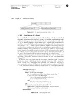
Figure 4.9 shows an example of C code using the
ODBC API. The first step in using
ODBC to communicate with a server is to set up a connection with the server. To do
so, the program first allocates an SQL environment, then a database connection han-
dle.
ODBC defines the types HENV, HDBC,andRETCODE. The program then opens
the database connection by using

SQLConnect. This call takes several parameters, in-
Silberschatz−Korth−Sudarshan:

Database System
Concepts, Fourth Edition
II. Relational Databases 4. SQL
183
© The McGraw−Hill
Companies, 2001
4.13 Dynamic SQL 177
int ODBCexample()
{
RETCODE error;
HENV env; /* environment */
HDBC conn; /* database connection */
SQLAllocEnv(&env);
SQLAllocConnect(env, &conn);
SQLConnect(conn, ”aura.bell-labs.com”, SQL NTS,”avi”,SQL NTS,
”avipasswd”,
SQL NTS);
{
char branchname[80];
float balance;
int lenOut1, lenOut2;
HSTMT stmt;
SQLAllocStmt(conn, &stmt);
char * sqlquery = ”select branch
name, s um (balance)
from account
group by branch

name”;
error =
SQLExecDirect(stmt, sqlquery, SQL NTS);
if (error ==
SQL SUCCESS) {
SQLBindCol(stmt, 1, SQL C CHAR, branchname , 80, &lenOut1);
SQLBindCol(stmt, 2, SQL C FLOAT, &balance, 0 , &lenOut2);
while (
SQLFetch(stmt) >= SQL SUCCESS) {
printf (” %s %g\n”, branchname, balance);
}
}
}
SQLFreeStmt(stmt, SQL DROP);
SQLDisconnect(conn);
SQLFreeConnect(conn);
SQLFreeEnv(env);
}
Figure 4.9
ODBC code example.
cluding the connection handle, the server to which to connect, the user identifier,
and the password for the database. The constant
SQL NTS denotes that the previous
argument is a null-terminated string.
Once the connection is set up, the program can send
SQL commands to the database
by using
SQLExecDirect C language variables can be bound to attributes of the query
result, so that when a result tuple is fetched using
SQLFetch, its attribute values are

stored in corresponding C variables. The
SQLBindCol function does this task; the sec-
ond argument identifies the position of the attribute in the query result, and the third
argument indicates the type conversion required from
SQL to C. The next argument
Silberschatz−Korth−Sudarshan:

Database System
Concepts, Fourth Edition
II. Relational Databases 4. SQL
184
© The McGraw−Hill
Companies, 2001
178 Chapter 4 SQL
gives the address of the variable. For variable-length types like character arrays, the
last two arguments give the maximum length of the variable and a location where
the actual length is to be stored when a tuple is fetched. A negative value returned
for the length field indicates that the value is null.
The
SQLFetch statement is in a while loop that gets executed until SQLFetch re-
turns a value other than
SQL SUCCESS. On each fetch, the program stores the values
in C variables as specified by the calls on
SQLBindCol and prints out these values.
At the end of the session, the program frees the statement handle, disconnects
from the database, and frees up the connection and
SQL environment handles. Good
programming style requires that the result of every function call must be checked to
make sure there are no errors; we have omitted most of these checks for brevity.
It is possible to create an

SQL statement with parameters; for example, consider
the statement insert into account values(?,?,?). The question marks are placeholders
for values which will be supplied later. The above statement can be “prepared,” that
is, compiled at the database, and repeatedly executed by providing actual values for
the placeholders—in this case, by providing an account number, branch name, and
balancefortherelationaccount.
ODBC defines functions for a variety of tasks, such as finding all the relations in the
database and finding the names and types of columns of a query result or a relation
in the database.
By default, each
SQL statement is treated as a separate transaction that is commit-
ted automatically. The call
SQLSetConnectOption(conn, SQL AUTOCOMMIT, 0) turns
off automatic commit on connection
conn, and transactions must then be committed
explicitly by
SQLTransact(conn, SQL COMMIT) or rolled back by SQLTransact(conn,
SQL ROLLBACK).
The more recent versions of the
ODBC standard add new functionality. Each ver-
sion defines conformance levels, which specify subsets of the functionality defined by
the standard. An
ODBC implementation may provide only core level features, or it
may provide more advanced (level 1 or level 2) features. Level 1 requires support
for fetching information about the catalog, such as information about what relations
are present and the types of their attributes. Level 2 requires further features, such as
ability to send and retrieve arrays of parameter values and to retrieve more detailed
catalog information.
The more recent
SQL standards (SQL-92 and SQL:1999)defineacall level interface

(CLI) that is similar to the
ODBC interface, but with some minor differences.
4.13.2 JDBC∗∗
The JDBC standard defines an API that Java programs can use to connect to database
servers. (The word
JDBC was originally an abbreviation for “Java Database Connec-
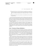
tivity”, but the full form is no longer used.) Figure 4.10 shows an example Java pro-
gram that uses the
JDBC interface. The program must first open a connection to a
database, and can then execute
SQL statements, but before opening a connection,
it loads the appropriate drivers for the database by using
Class.forName. The first
parameter to the getConnection call specifies the machine name where the server
Silberschatz−Korth−Sudarshan:

Database System
Concepts, Fourth Edition
II. Relational Databases 4. SQL
185
© The McGraw−Hill
Companies, 2001
4.13 Dynamic SQL 179
public static void JDBCexample(String dbid, String userid, String passwd)
{
try
{
Class.forName (”oracle.jdbc.driver.OracleDriver”);
Connection conn = DriverManager.getConnection(
”jdbc:oracle:thin:@aur a.bell-labs.com:2000:bankdb”,

userid, passwd);
Statement stmt = conn.createStatement();
try {
stmt.executeUpdate(
”insert into account values(’A-9732’, ’Perryridge’, 1200)”);
} catch (
SQLException sqle)
{
System.out.println(”Could not insert tuple. ” + sqle);
}
ResultSet rset = stmt.executeQuery(
”select branch
name, avg (balance)
from account
group by branch
name”);
while (rset.next()) {
System.out.println(rset.getString(”branch
name”) + ” ” +
rset.getFloat(2));
}
stmt.close();
conn.close();
}
catch (
SQLException sqle)
{
System.out.println(”SQLException : ” + sqle);
}
}

Figure 4.10 An example of
JDBC code.
runs (in our example, aura.bell-labs.com), the port number it uses for communica-
tion (in our example, 2000). The parameter also specifies which schema on the server
is to be used (in our example, bankdb), since a database server may support multiple
schemas. The first parameter also specifies the protocol to be used to communicate
with the database (in our example, jdbc:oracle:thin:). Note that
JDBC specifies only
the
API, not the communication protocol. A JDBC driver may support multiple pro-
tocols, and we must specify one supported by both the database and the driver. The
other two arguments to getConnection are a user identifier and a password.
The program then creates a statement handle on the connection and uses it to
execute an
SQL statement and get back results. In our example, stmt.executeUpdate
executes an update statement. The try { } catch { } construct permits us to
Silberschatz−Korth−Sudarshan:

Database System
Concepts, Fourth Edition
II. Relational Databases 4. SQL
186
© The McGraw−Hill
Companies, 2001
180 Chapter 4 SQL
PreparedStatement pStmt = conn.prepareStatement(
”insert into account values(?,?,?)”);
pStmt.setString(1, ”A-9732”);
pStmt.setString(2, ”Perryridge”);
pStmt.setInt(3, 1200);

pStmt.executeUpdate();
pStmt.setString(1, ”A-9733”);
pStmt.executeUpdate();
Figure 4.11 Prepared statements in JDBC code.
catch any exceptions (error conditions) that arise when
JDBC calls are made, and print
an appropriate message to the user.
The program can execute a query by using stmt.execute
Query. It can retrieve the
set of rows in the result into a
ResultSet and fetch them one tuple at a time using the
next() function on the result set. Figure 4.10 shows two ways of retrieving the values
of attributes in a tuple: using the name of the attribute (branch-name) and using the
position of the attribute (2, to denote the second attribute).
We can also create a prepared statement in which some values are replaced by “?”,
thereby specifying that actual values will be provided later. We can then provide the
values by using set
String(). The database can compile the query when it is prepared,
and each time it is executed (with new values), the database can reuse the previously
compiled form of the query. The code fragment in Figure 4.11 shows how prepared
statements can be used.
JDBC provides a number of other features, such as updatable result sets.Itcan
create an updatable result set from a query that performs a selection and/or a pro-
jection on a database relation. An update to a tuple in the result set then results in
an update to the corresponding tuple of the database relation.
JDBC also provides an
API to examine database schemas and to find the types of attributes of a result set.
For more information about
JDBC, refer to the bibliographic information at the end
of the chapter.

4.14 Other SQL Features ∗∗
The SQL language has grown over the past two decades from a simple language with
a few features to a rather complex language with features to satisfy many different
types of users. We covered the basics of
SQL earlier in this chapter. In this section we
introduce the reader to some of the more complex features of
SQL.
4.14.1 Schemas, Catalogs, and Environments
To understand the motivation for schemas and catalogs, consider how files are named
in a file system. Early file systems were flat; that is, all files were stored in a single
directory. Current generation file systems of course have a directory structure, with
Silberschatz−Korth−Sudarshan:

Database System
Concepts, Fourth Edition
II. Relational Databases 4. SQL
187
© The McGraw−Hill
Companies, 2001
4.14 Other SQL Features ∗∗ 181
files stored within subdirectories. To name a file uniquely, we must specify the full
path name of the file, for example, /users/avi/db-book/chapter4.tex.
Like early file systems, early database systems also had a single name space for all
relations. Users had to coordinate to make sure they did not try to use the same name
for different relations. Contemporary database systems provide a three-level hierar-
chy for naming relations. The top level of the hierarchy consists of catalogs,eachof
which can contain schemas.
SQL objects such as relations and views are contained
within a schema.
In order to perform any actions on a database, a user (or a program) must first

connect to the database. The user must provide the user name and usually, a secret
password for verifying the identity of the user, as we saw in the
ODBC and JDBC
examples in Sections 4.13.1 and 4.13.2. Each user has a default catalog and schema,
and the combination is unique to the user. When a user connects to a database system,
the default catalog and schema are set up for for the connection; this corresponds to
the current directory being set to the user’s home directory when the user logs into
an operating system.
To identify a relation uniquely, a three-part name must be used, for example,
catalog5.bank-schema.account
We may omit the catalog component, in which case the catalog part of the name is
considered to be the default catalog for the connection. Thus if catalog5 is the default
catalog, we can use bank-schema.account to identify the same relation uniquely. Fur-
ther, we may also omit the schema name, and the schema part of the name is again
considered to be the default schema for the connection. Thus we can use just account
if the default catalog is catalog5 and the default schema is bank-schema.
With multiple catalogs and schemas available, different applications and differ-
ent users can work independently without worrying about name clashes. Moreover,
multiple versions of an application—one a production version, other test versions—
can run on the same database system.
The default catalog and schema are part of an
SQL environment that is set up
for each connection. The environment additionally contains the user identifier (also
referred to as the authorization identifier). All the usual
SQL statements, including the
DDL and DML statements, operate in the context of a schema. We can create and
drop schemas by means of create schema and drop schema statements. Creation and
dropping of catalogs is implementation dependent and not part of the
SQL standard.
4.14.2 Procedural Extensions and Stored Procedures

SQL provides a module language, which allows procedures to be defined in SQL.
A module typically contains multiple
SQL procedures. Each procedure has a name,
optional arguments, and an
SQL statement. An extension of the SQL-92 standard lan-
guage also permits procedural constructs, such as for, while,andif-then-else,and
compound
SQL statements (multiple SQL statements between a begin and an end).
We can store procedures in the database and then execute them by using the call
statement. Such procedures are also called stored procedures. Stored procedures
Silberschatz−Korth−Sudarshan:

Database System
Concepts, Fourth Edition
II. Relational Databases 4. SQL
188
© The McGraw−Hill
Companies, 2001
182 Chapter 4 SQL
are particularly useful because they permit operations on the database to be made
available to external applications, without exposing any of the internal details of the
database.
Chapter 9 covers procedural extensions of
SQL as well as many other new features
of
SQL:1999.
4.15 Summary
• Commercial database systems do not use the terse, formal query languages
covered in Chapter 3. The widely used
SQL language, which we studied in

this chapter, is based on the formal relational algebra, but includes much “syn-
tactic sugar.”
•
SQL includes a variety of language constructs for queries on the database. All
the relational-algebra operations, including the extended relational-algebra
operations, can be expressed by
SQL. SQL also allows ordering of query re-
sults by sorting on specified attributes.
• View relations can be defined as relations containing the result of queries.
Views are useful for hiding unneeded information, and for collecting together
information from more than one relation into a single view.
• Temporary views defined by using the with clause are also useful for breaking
up complex queries into smaller and easier-to-understand parts.
•
SQL provides constructs for updating, inserting, and deleting information. A
transaction consists of a sequence of operations, which must appear to be
atomic. That is, all the operations are carried out successfully, or none is car-
ried out. In practice, if a transaction cannot complete successfully, any partial
actions it carried out are undone.
• Modifications to the database may lead to the generation of null values in
tuples. We discussed how nulls can be introduced, and how the
SQL query
language handles queries on relations containing null values.
• The
SQL data definition language is used to create relations with specified
schemas. The
SQL DDL supports a number of types including date and time
types. Further details on the
SQL DDL, in particular its support for integrity
constraints, appear in Chapter 6.

•
SQL queries can be invoked from host languages, via embedded and dynamic
SQL.TheODBC and JDBC standards define application program interfaces to
access
SQL databases from C and Java language programs. Increasingly, pro-
grammers use these
APIs to access databases.
• We also saw a brief overview of some advanced features of
SQL,suchaspro-
cedural extensions, catalogs, schemas and stored procedures.
Silberschatz−Korth−Sudarshan:

Database System
Concepts, Fourth Edition
II. Relational Databases 4. SQL
189
© The McGraw−Hill
Companies, 2001
Exercises 183
Review Terms
• DDL: data definition language
• DML: data manipulation
language
• select clause
• from clause
• where clause
• as clause
• Tuple variable
• order by clause
• Duplicates

• Set operations
union, intersect, except
• Aggregate functions
avg, min, max, sum, count
group by
• Null values
Truth value “unknown”
• Nested subqueries
• Set operations
{<, <=,>,>=}{some, all }
exists
unique
• Views
• Derived relations (in from clause)
• with clause
• Database modification
delete, insert, update
View update
• Join types
Inner and outer join
left, right and full outer join
natural, using, and on
• Transaction
• Atomicity
• Index
• Schema
• Domains
• Embedded SQL
• Dynamic SQL
• ODBC

• JDBC
• Catalog
• Stored procedures
Exercises
4.1 Consider the insurance database of Figure 4.12, where the primary keys are un-
derlined. Construct the following
SQL queries for this relational database.
a. Find the total number of people who owned cars that were involved in ac-
cidents in 1989.
b. Find the number of accidents in which the cars belonging to “John Smith”
were involved.
c. Add a new accident to the database; assume any values for required at-
tributes.
d. Delete the Mazda belonging to “John Smith”.
e. Update the damage amount for the car with license number “AABB2000” in
the accident with report number “AR2197” to $3000.
4.2 Consider the employee database of Figure 4.13, where the primary keys are un-
derlined. Give an expression in
SQL for each of the following queries.
a. Find the names of all employees who work for First Bank Corporation.
Silberschatz−Korth−Sudarshan:

Database System
Concepts, Fourth Edition
II. Relational Databases 4. SQL
190
© The McGraw−Hill
Companies, 2001
184 Chapter 4 SQL
person (driver-id#, name, address)

car (license
, model, year)
accident (report-number
, date, location)
owns (driver-id#
, license)
participated (driver-id
, car, report-number, damage-amount)
Figure 4.12 Insurance database.
employee (employee-name
, street, city)
works (employee-name
, company-name, salary)
company (company-name
, city)
manages (employee-name
, manager-name)
Figure 4.13 Employee database.
b. Find the names and cities of residence of all employees who work for First
Bank Corporation.
c. Find the names, street addresses, and cities of residence of all employees
who work for First Bank Corporation and earn more than $10,000.
d. Find all employees in the database who live in the same cities as the com-
panies for which they work.
e. Find all employees in the database who live in the same cities and on the
same streets as do their managers.
f. Find all employees in the database who do not work for First Bank Corpo-
ration.
g. Find all employees in the database who earn more than each employee of
Small Bank Corporation.

h. Assume that the companies may be located in several cities. Find all com-
panies located in every city in which Small Bank Corporation is located.
i. Find all employees who earn more than the average salary of all employees
of their company.
j. Find the company that has the most employees.
k. Find the company that has the smallest payroll.
l. Find those companies whose employees earn a higher salary, on average,
than the average salary at First Bank Corporation.
4.3 Consider the relational database of Figure 4.13. Give an expression in
SQL for
each of the following queries.
a. Modify the database so that Jones now lives in Newtown.
b. Give all employees of First Bank Corporation a 10 percent raise.
c. Give all managers of First Bank Corporation a 10 percent raise.
d. Give all managers of First Bank Corporation a 10 percent raise unless the
salary becomes greater than $100,000; in such cases, give only a 3 percent
raise.
e. Delete all tuples in the works relation for employees of Small Bank Corpora-
tion.
Silberschatz−Korth−Sudarshan:

Database System
Concepts, Fourth Edition
II. Relational Databases 4. SQL
191
© The McGraw−Hill
Companies, 2001
Exercises 185
4.4 Let the following relation schemas be given:
R =(A, B, C)

S =(D,E, F)
Let relations r(R)ands(S) be given. Give an expression in
SQL that is equivalent
to each of the following queries.
a. Π
A
(r)
b. σ
B =17
(r)
c. r × s
d. Π
A,F
(σ
C = D
(r × s))
4.5 Let R =(A, B, C),andletr
1
and r
2
both be relations on schema R.Givean
expression in
SQL that is equivalent to each of the following queries.
a. r
1
∪ r
2
b. r
1
∩ r

2
c. r
1
− r
2
d. Π
AB
(r
1
) Π
BC
(r
2
)
4.6 Let R =(A, B) and S =(A, C),andletr(R) and s(S) be relations. Write an
expression in
SQL for each of the queries below:
a. {<a> |∃b (<a,b>∈ r ∧ b = 17)}
b. {<a,b,c> | <a,b>∈ r ∧ <a,c>∈ s}
c. {<a> |∃c (<a,c>∈ s ∧∃b
1
,b
2
(<a,b
1
> ∈ r ∧ <c,b
2
> ∈ r ∧ b
1
>

b
2
))}
4.7 Show that, in
SQL, <> all is identical to not in.
4.8 Consider the relational database of Figure 4.13. Using
SQL, define a view con-
sisting of manager-name and the average salary of all employees who work for
that manager. Explain why the database system should not allow updates to be
expressed in terms of this view.
4.9 Consider the
SQL query
select p.a1
from p, r1, r2
where p.a1 = r1.a1 or p.a1 = r2.a1
Under what conditions does the preceding query select values of p.a1 that are
either in r1 or in r2? Examine carefully the cases where one of r1 or r2 may be
empty.
4.10 Write an
SQL query, without using a with clause, to find all branches where
the total account deposit is less than the average total account deposit at all
branches,
a. Using a nested query in the from clauser.
Silberschatz−Korth−Sudarshan:

Database System
Concepts, Fourth Edition
II. Relational Databases 4. SQL
192
© The McGraw−Hill

Companies, 2001
186 Chapter 4 SQL
b. Using a nested query in a having clause.
4.11 Suppose that we have a relation marks(student-id, score) and we wish to assign
grades to students based on the score as follows: grade F if score < 40,gradeC
if 40 ≤ score < 60,gradeB if 60 ≤ score < 80,andgradeA if 80 ≤ score.Write
SQL queries to do the following:
a. Display the grade for each student, based on the marks relation.
b. Find the number of students with each grade.
4.12
SQL-92 provides an n-ary operation called coalesce, which is defined as follows:
coalesce(A
1
,A
2
, ,A
n
) returns the first nonnull A
i
in the list A
1
,A
2
, ,A
n
,
and returns null if all of A
1
,A
2

, ,A
n
are null. Show how to express the coa-
lesce operation using the case operation.
4.13 Let a and b be relations with the schemas A(name, address, title) and B(name, ad-
dress, salary), respectively. Show how to express a natural full outer join b using
the full outer join operation with an on condition and the coalesce operation.
Make sure that the result relation does not contain two copies of the attributes
name and address, and that the solution is correct even if some tuples in a and b
have null values for attributes name or address.
4.14 Give an
SQL schema definition for the employee database of Figure 4.13. Choose
an appropriate domain for each attribute and an appropriate primary key for
each relation schema.
4.15 Write check conditions for the schema you defined in Exercise 4.14 to ensure
that:
a. Every employee works for a company located in the same city as the city in
which the employee lives.
b. No employee earns a salary higher than that of his manager.
4.16 Describe the circumstances in which you would choose to use embedded
SQL
rather than SQL alone or only a general-purpose programming language.
Bibliographical Notes
The original version of SQL, called Sequel 2, is described by Chamberlin et al. [1976].
Sequel 2 was derived from the languages Square Boyce et al. [1975] and Chamber-
lin and Boyce [1974]. The American National Standard
SQL-86 is described in ANSI
[1986]. The
IBM Systems Application Architecture definition of SQL is defined by IBM
[1987]. The official standards for

SQL-89 and SQL-92 are available as ANSI [1989] and
ANSI [1992], respectively.
Textbook descriptions of the
SQL-92 language include Date and Darwen [1997],
Melton and Simon [1993], and Cannan and Otten [1993]. Melton and Eisenberg [2000]
provides a guide to
SQLJ, JDBC, and related technologies. More information on SQLJ
and SQLJ software can be obtained from . Date and Darwen [1997]
and Date [1993a] include a critique of
SQL-92.
Silberschatz−Korth−Sudarshan:

Database System
Concepts, Fourth Edition
II. Relational Databases 4. SQL
193
© The McGraw−Hill
Companies, 2001
Bibliographical Notes 187
Eisenberg and Melton [1999] provide an overview of SQL:1999.Thestandardis
published as a sequence of five ISO/IEC standards documents, with several more
parts describing various extensions under development. Part 1 (SQL/Framework),
gives an overview of the other parts. Part 2 (SQL/Foundation) outlines the basics of
the language. Part 3 (SQL/CLI) describes the Call-Level Interface. Part 4 (SQL/PSM)
describes Persistent Stored Modules, and Part 5 (SQL/Bindings) describes host lan-
guage bindings. The standard is useful to database implementers but is very hard
to read. If you need them, you can purchase them electronically from the Web site
.
Many database products support
SQL features beyond those specified in the stan-

dards, and may not support some features of the standard. More information on
these features may be found in the
SQL user manuals of the respective products.
is an excellent source for more (and up-to-
date) information on
JDBC, and on Java in general. References to books on Java (in-
cluding
JDBC) are also available at this URL.TheODBC API is described in Microsoft
[1997] and Sanders [1998].
The processing of
SQL queries, including algorithms and performance issues, is
discussed in Chapters 13 and 14. Bibliographic references on these matters appear in
that chapter.
Silberschatz−Korth−Sudarshan:

Database System
Concepts, Fourth Edition
II. Relational Databases 5. Other Relational
Languages
194
© The McGraw−Hill
Companies, 2001
CHAPTER 5
Other Relational Languages
In Chapter 4, we described SQL—the most influential commercial relational-database
language. In this chapter, we study two more languages:
QBE and Datalog. Unlike
SQL, QBE is a graphical language, where queries look like tables. QBE and its variants
are widely used in database systems on personal computers. Datalog has a syntax
modeled after the Prolog language. Although not used commercially at present, Dat-

alog has been used in several research database systems.
Here, we present fundamental constructs and concepts rather than a complete
users’ guide for these languages. Keep in mind that individual implementations of a
language may differ in details, or may support only a subset of the full language.
In this chapter, we also study forms interfaces and tools for generating reports and
analyzing data. While these are not strictly speaking languages, they form the main
interface to a database for many users. In fact, most users do not perform explicit
querying with a query language at all, and access data only via forms, reports, and
other data analysis tools.
5.1 Query-by-Example
Query-by-Example (QBE) is the name of both a data-manipulation language and an
early database system that included this language. The
QBE database system was
developed at
IBM’s T. J. Watson Research Center in the early 1970s. The QBE data-
manipulation language was later used in
IBM’s Query Management Facility (QMF).
Today, many database systems for personal computers support variants of
QBE lan-
guage. In this section, we consider only the data-manipulation language. It has two
distinctive features:
1. Unlike most query languages and programming languages,
QBE has a two-
dimensional syntax:Querieslook like tables. A query in a one-dimensional
189
Silberschatz−Korth−Sudarshan:

Database System
Concepts, Fourth Edition
II. Relational Databases 5. Other Relational

Languages
195
© The McGraw−Hill
Companies, 2001
190 Chapter 5 Other Relational Languages
language (for example, SQL) can be written in one (possibly long) line. A two-
dimensional language requires two dimensions for its expression. (There is a
one-dimensional version of
QBE, but we shall not consider it in our discus-
sion).
2.
QBE queries are expressed “by example.” Instead of giving a procedure for
obtaining the desired answer, the user gives an example of what is desired.
The system generalizes this example to compute the answer to the query.
Despite these unusual features, there is a close correspondence between
QBE and the
domain relational calculus.
We express queries in
QBE by skeleton tables. These tables show the relation
schema, as in Figure 5.1. Rather than clutter the display with all skeletons, the user se-
lects those skeletons needed for a given query and fills in the skeletons with example
rows. An example row consists of constants and example elements, which are domain
variables. To avoid confusion between the two,
QBE uses an underscore character ( )
before domain variables, as in
x, and lets constants appear without any qualification.
branch branch-name branch-city assets
customer customer-name customer-street customer-city
loan loan-number branch-name amount
borrower customer-name loan-number

account account-number branch-name balance
depositor customer-name account-number
Figure 5.1 QBE skeleton tables for the bank example.
Silberschatz−Korth−Sudarshan:

Database System
Concepts, Fourth Edition
II. Relational Databases 5. Other Relational
Languages
196
© The McGraw−Hill
Companies, 2001
5.1 Query-by-Example 191
This convention is in contrast to those in most other languages, in which constants
are quoted and variables appear without any qualification.
5.1.1 Queries on One Relation
Returning to our ongoing bank example, to find all loan numbers at the Perryridge
branch, we bring up the skeleton for the loan relation, and fill it in as follows:
loan loan-number branch-name amount
P. x Perryridge
This query tells the system to look for tuples in
loan that have “Perryridge” as the
value for the branch-name attribute. For each such tuple, the system assigns the value
of the loan-number attribute to the variable x.It“prints” (actually, displays) the value
of the variable x, because the command P. appears in the loan-number column next to
the variable x. Observe that this result is similar to what would be done to answer
the domain-relational-calculus query
{x|∃b, a(x, b, a∈loan ∧ b = “Perryridge”)}
QBE assumes that a blank position in a row contains a unique variable. As a result,
if a variable does not appear more than once in a query, it may be omitted. Our

previous query could thus be rewritten as
loan loan-number branch-name amount
P. Perryridge
QBE (unlike SQL) performs duplicate elimination automatically. To suppress du-
plicate elimination, we insert the command ALL. after the P. command:
loan loan-number branch-name amount
P.ALL. Perryridge
To display the entire loan relation, we can create a single row consisting of P. in
every field. Alternatively, we can use a shorthand notation by placing a single P. in
the column headed by the relation name:
loan loan-number branch-name amount
P.
QBE allows queries that involve arithmetic comparisons (for example, >), rather
than equality comparisons, as in “Find the loan numbers of all loans with a loan
amount of more than $700”:
loan loan-number branch-name amount
P. >700
Silberschatz−Korth−Sudarshan:

Database System
Concepts, Fourth Edition
II. Relational Databases 5. Other Relational
Languages
197
© The McGraw−Hill
Companies, 2001
192 Chapter 5 Other Relational Languages
Comparisons can involve only one arithmetic expression on the right-hand side of
the comparison operation (for example, > (
x + y −20)). The expression can include

both variables and constants. The space on the left-hand side of the comparison op-
eration must be blank. The arithmetic operations that
QBE supports are =, <, ≤, >,
≥,and¬.
Note that requiring the left-hand side to be blank implies that we cannot compare
two distinct named variables. We shall deal with this difficulty shortly.
As yet another example, consider the query “Find the names of all branches that
are not located in Brooklyn.” This query can be written as follows:
branch branch-name branch-city assets
P. ¬ Brooklyn
The primary purpose of variables in QBE is to force values of certain tuples to have
the same value on certain attributes. Consider the query “Find the loan numbers of
allloansmadejointlytoSmithandJones”:
borrower customer-name loan-number
“Smith” P. x
“Jones” x
To execute this query, the system finds all pairs of tuples in borrower that agree on
the loan-number attribute, where the value for the customer-name attribute is “Smith”
for one tuple and “Jones” for the other. The system then displays the value of the
loan-number attribute.
In the domain relational calculus, the query would be written as
{l|∃x (x, l∈borrower ∧ x = “Smith”)
∧∃x (x, l∈borrower ∧ x = “Jones”)}
As another example, consider the query “Find all customers who live in the same
city as Jones”:
customer customer-name customer-street customer-city
P. x y
Jones y
5.1.2 Queries on Several Relations
QBE allows queries that span several different relations (analogous to Cartesian prod-

uct or natural join in the relational algebra). The connections among the various rela-
tions are achieved through variables that force certain tuples to have the same value
on certain attributes. As an illustration, suppose that we want to find the names of all
customers who have a loan from the Perryridge branch. This query can be written as
Silberschatz−Korth−Sudarshan:

Database System
Concepts, Fourth Edition
II. Relational Databases 5. Other Relational
Languages
198
© The McGraw−Hill
Companies, 2001
5.1 Query-by-Example 193
loan loan-number branch-name amount
x Perryridge
borrower customer-name loan-number
P. y x
To evaluate the preceding query, the system finds tuples in loan with “Perryridge”
as the value for the branch-name attribute. For each such tuple, the system finds tu-
ples in borrower with the same value for the loan-number attribute as the loan tuple. It
displays the values for the customer-name attribute.
We can use a technique similar to the preceding one to write the query “Find the
names of all customers who have both an account and a loan at the bank”:
depositor customer-name account-number
P. x
borrower customer-name loan-number
x
Now consider the query “Find the names of all customers who have an account
at the bank, but who do not have a loan from the bank.” We express queries that

involve negation in
QBE by placing a not sign (¬) under the relation name and next
to an example row:
depositor customer-name account-number
P. x
borrower customer-name loan-number
x
¬
Compare the preceding query with our earlier query “Find the names of all cus-
tomerswhohavebothanaccountandaloanatthebank.” The only difference is the ¬
appearing next to the example row in the borrower skeleton. This difference, however,
has a major effect on the processing of the query.
QBE finds all x values for which
1. There is a tuple in the depositor relation whose customer-name is the domain
variable x.
2. There is no tuple in the borrower relation whose customer-name isthesameas
in the domain variable x.
The ¬ can be read as “there does not exist.”
The fact that we placed the ¬ under the relation name, rather than under an at-
tribute name, is important. A ¬ under an attribute name is shorthand for =.Thus,to
find all customers who have at least two accounts, we write
Silberschatz−Korth−Sudarshan:

Database System
Concepts, Fourth Edition
II. Relational Databases 5. Other Relational
Languages
199
© The McGraw−Hill
Companies, 2001

194 Chapter 5 Other Relational Languages
depositor customer-name account-number
P. x y
x ¬ y
In English, the preceding query reads “Display all customer-name values that ap-
pear in at least two tuples, with the second tuple having an account-number different
from the first.”
5.1.3 The Condition Box
At times, it is either inconvenient or impossible to express all the constraints on the
domain variables within the skeleton tables. To overcome this difficulty,
QBE includes
a condition box feature that allows the expression of general constraints over any of
the domain variables.
QBE allows logical expressions to appear in a condition box.
The logical operators are the words and and or,orthesymbols“&” and “|”.
For example, the query “Find the loan numbers of all loans made to Smith, to Jones
(or to both jointly)” canbewrittenas
borrower customer-name loan-number
n P. x
conditions
n = Smith or n = Jones
It is possible to express the above query without using a condition box, by using
P. in multiple rows. However, queries with P. in multiple rows are sometimes hard to
understand, and are best avoided.
As yet another example, suppose that we modify the
final query in Section 5.1.2
to be “Find all customers who are not named ‘Jones’ and who have at least two ac-
counts.” We want to include an “x = Jones” constraint in this query. We do that by
bringing up the condition box and entering the constraint “x ¬ = Jones”:
conditions

x ¬ = Jones
Turning to another example, to find all account numbers with a balance between
$1300 and $1500, we write
account account-number branch-name balance
P. x
conditions
x ≥ 1300
x ≤ 1500
Silberschatz−Korth−Sudarshan:

Database System
Concepts, Fourth Edition
II. Relational Databases 5. Other Relational
Languages
200
© The McGraw−Hill
Companies, 2001
5.1 Query-by-Example 195
As another example, consider the query “Find all branches that have assets greater
than those of at least one branch located in Brooklyn.” This query can be written as
branch branch-name branch-city assets
P. x y
Brooklyn z
conditions
y > z
QBE allows complex arithmetic expressions to appear in a condition box. We can
write the query “Find all branches that have assets that are at least twice as large as
the assets of one of the branches located in Brooklyn” much as we did in the preced-
ing query, by modifying the condition box to
conditions

y ≥ 2* z
To find all account numbers of account with a balance between $1300 and $2000,
but not exactly $1500, we write
account account-number branch-name balance
P. x
x
conditions
( ≥ 1300 ≤ 2000 ¬ 1500)and and
=
QBE uses the or construct in an unconventional way to allow comparison with a set
of constant values. To find all branches that are located in either Brooklyn or Queens,
we write
branch branch-name branch-city assets
P. x
x = (Brooklyn or Queens)
conditions
5.1.4 The Result Relation
The queries that we have written thus far have one characteristic in common: The
results to be displayed appear in a single relation schema. If the result of a query
includes attributes from several relation schemas, we need a mechanism to display
the desired result in a single table. For this purpose, we can declare a temporary result
relation that includes all the attributes of the result of the query. We print the desired
result by including the command P. in only the result skeleton table.
Silberschatz−Korth−Sudarshan:

Database System
Concepts, Fourth Edition
II. Relational Databases 5. Other Relational
Languages
201

© The McGraw−Hill
Companies, 2001
196 Chapter 5 Other Relational Languages
As an illustration, consider the query “Find the customer-name, account-number,and
balance for all accounts at the Perryridge branch.” In relational algebra, we would
construct this query as follows:
1. Join depositor and account.
2. Project customer-name, account-number,andbalance.
To construct the same query in
QBE, we proceed as follows:
1. Create a skeleton table, called result, with attributes customer-name, account-
number,andbalance. The name of the newly created skeleton table (that is,
result) must be different from any of the previously existing database relation
names.
2. Write the query.
The resulting query is
account account-number branch-name balance
y Perryridge z
depositor customer-name account-number
x y
result customer-name account-number balance
P. x y z
5.1.5 Ordering of the Display of Tuples
QBE offers the user control over the order in which tuples in a relation are displayed.
We gain this control by inserting either the command
AO. (ascending order) or the
command
DO. (descending order) in the appropriate column. Thus, to list in ascend-
ing alphabetic order all customers who have an account at the bank, we write
depositor customer-name account-number

P. A O .
QBE provides a mechanism for sorting and displaying data in multiple columns.
We specify the order in which the sorting should be carried out by including, with
each sort operator (
AO or DO), an integer surrounded by parentheses. Thus, to list all
account numbers at the Perryridge branch in ascending alphabetic order with their
respective account balances in descending order, we write
account account-number branch-name balance
P. A O (1). Perryridge P. D O (2).
Silberschatz−Korth−Sudarshan:

Database System
Concepts, Fourth Edition
II. Relational Databases 5. Other Relational
Languages
202
© The McGraw−Hill
Companies, 2001
5.1 Query-by-Example 197
The command P. A O (1). specifies that the account number should be sorted first;
the command
P. D O (2). specifies that the balances for each account should then be
sorted.
5.1.6 Aggregate Operations
QBE includes the aggregate operators AV G, MAX, MIN, SUM,andCNT.Wemustpost-
fix these operators with
ALL. to create a multiset on which the aggregate operation is
evaluated. The
ALL. operator ensures that duplicates are not eliminated. Thus, to find
the total balance of all the accounts maintained at the Perryridge branch, we write

account account-number branch-name balance
Perryridge P.SUM.ALL.
We use the operator UNQ to specify that we want duplicates eliminated. Thus, to
find the total number of customers who have an account at the bank, we write
depositor customer-name account-number
P. C N T. U N Q .
QBE also offers the ability to compute functions on groups of tuples using the G.
operator, which is analogous to
SQL’s group by construct. Thus, to find the average
balance at each branch, we can write
account account-number branch-name balance
P. G . P.AVG.ALL. x
The average balance is computed on a branch-by-branch basis. The keyword ALL.
in the P. AV G . A L L .entryinthebalance column ensures that all the balances are consid-
ered. If we wish to display the branch names in ascending order, we replace
P. G . by
P. A O . G .
To find the average account balance at only those branches where the average
account balance is more than $1200, we add the following condition box:
conditions
AVG.ALL. x > 1200
As another example, consider the query “Find all customers who have accounts at
each of the branches located in Brooklyn”:
Silberschatz−Korth−Sudarshan:

Database System
Concepts, Fourth Edition
II. Relational Databases 5. Other Relational
Languages
203

© The McGraw−Hill
Companies, 2001
198 Chapter 5 Other Relational Languages
depositor customer-name account-number
P. G . x y
account account-number branch-name balance
y z
branch branch-name branch-city assets
z Brooklyn
w Brooklyn
conditions
CNT.UNQ. z =
CNT.UNQ. w
The domain variable w can hold the value of names of branches located in Brook-
lyn. Thus,
CNT.UNQ. w is the number of distinct branches in Brooklyn. The domain
variable z can hold the value of branches in such a way that both of the following
hold:
• The branch is located in Brooklyn.
• The customer whose name is x has an account at the branch.
Thus,
CNT.UNQ. z is the number of distinct branches in Brooklyn at which customer x
has an account. If
CNT.UNQ. z = CNT.UNQ. w,thencustomerx must have an account
at all of the branches located in Brooklyn. In such a case, the displayed result includes
x (because of the
P. ).
5.1.7 Modification of the Database
In this section, we show how to add, remove, or change information in QBE.
5.1.7.1 Deletion

Deletion of tuples from a relation is expressed in much the same way as a query. The
major difference is the use of D. in place of P.
QBE (unlike SQL), lets us delete whole
tuples, as well as values in selected columns. When we delete information in only
some of the columns, null values, specified by −,areinserted.
We note that a D. command operates on only one relation. If we want to delete
tuples from several relations, we must use one D. operator for each relation.
Here are some examples of
QBE delete requests:
• Delete customer Smith.
customer customer-name customer-street customer-city
D. Smith
Silberschatz−Korth−Sudarshan:

Database System
Concepts, Fourth Edition
II. Relational Databases 5. Other Relational
Languages
204
© The McGraw−Hill
Companies, 2001
5.1 Query-by-Example 199
• Delete the branch-city valueofthebranchwhosenameis“Perryridge.”
branch branch-name branch-city assets
Perryridge D.
Thus, if before the delete operation the
branch relation contains the tuple
(Perryridge, Brooklyn, 50000), the delete results in the replacement of the pre-
ceding tuple with the tuple (Perryridge, −, 50000).
• Delete all loans with a loan amount between $1300 and $1500.

loan loan-number branch-name amount
D. y x
borrower customer-name loan-number
D. y
conditions
x = (≥ 1300 ≤ 1500)and
Note that to delete loans we must delete tuples from both the loan and bor-
rower relations.
• Delete all accounts at all branches located in Brooklyn.
account account-number branch-name balance
D. y x
depositor customer-name account-number
D. y
branch branch-name branch-city assets
x Brooklyn
Note that, in expressing a deletion, we can reference relations other than those from
which we are deleting information.
5.1.7.2 Insertion
To insert data into a relation, we either specify a tuple to be inserted or write a query
whose result is a set of tuples to be inserted. We do the insertion by placing the I.
operator in the query expression. Obviously, the attribute values for inserted tuples
must be members of the attribute’s domain.
The simplest insert is a request to insert one tuple. Suppose that we wish to insert
the fact that account A-9732 at the Perryridge branch has a balance of $700. We write
Silberschatz−Korth−Sudarshan:

Database System
Concepts, Fourth Edition
II. Relational Databases 5. Other Relational
Languages

205
© The McGraw−Hill
Companies, 2001
200 Chapter 5 Other Relational Languages
account account-number branch-name balance
I. A-9732 Perryridge 700
We can also insert a tuple that contains only partial information. To insert infor-
mation into the
branch relation about a new branch with name “Capital” and city
“Queens,” but with a null asset value, we write
branch branch-name branch-city assets
I. Capital Queens
More generally, we might want to insert tuples on the basis of the result of a query.
Consider again the situation where we want to provide as a gift, for all loan cus-
tomers of the Perryridge branch, a new $200 savings account for every loan account
that they have, with the loan number serving as the account number for the savings
account. We write
account account-number branch-name balance
I. x Perryridge 200
depositor customer-name account-number
I. y x
loan loan-number branch-name amount
x Perryridge
borrower customer-name loan-number
y x
To execute the preceding insertion request, the system must get the appropriate
information from the borrower relation, then must use that information to insert the
appropriate new tuple in the depositor and account relations.
5.1.7.3 Updates
There are situations in which we wish to change one value in a tuple without chang-

ing all values in the tuple. For this purpose, we use the U. operator. As we could
for insert and delete, we can choose the tuples to be updated by using a query.
QBE,
however, does not allow users to update the primary key fields.
Suppose that we want to update the asset value of the of the Perryridge branch to
$10,000,000. This update is expressed as
branch branch-name branch-city assets
Perryridge U.10000000