FUNDAMENTALS OF DATABASE SYSTEMS Fourth Edition phần 4 pptx
Bạn đang xem bản rút gọn của tài liệu. Xem và tải ngay bản đầy đủ của tài liệu tại đây (3.84 MB, 103 trang )
296
IChapter 10 Functional Dependencies and
Normalization
for Relational Databases
EMPLOYEE
f.k.
I
ENAME
SSN
BDATE
ADDRESS
DNUMBER
p.k.
DEPARTMENT
I.k.
I
DNAME
DNUMBER
DMGRSSN
p.k.
DEPT_LOCATIONS
I.k.
DNUMBER
DLOCATION
y
p.k.
PROJECT
f.k.
I
PNAME
PNUMBER
PLOCATION
DNUM
p.k.
WORKS_ON
f.k.
I.k.
~
PNUMBER
~ ~y~ ~
I
HOURS
p.k.
FIGURE 10.1 A simplified
COMPANY
relational database schema.
The
semantics of the other two relation schemas in Figure 10.1 are slightly
more
complex. Each tuple in
DEPT_LOCATIONS
gives a department number
(DNUMBER)
and one of
the
locations of the department (DLOCATION). Each tuple in
WORKS_ON
gives an employee
social
security number (SSN), the project number of one of the projects
that
the employee
works
on
(PNUMBER),
and the number of hours per week
that
the employee works
on
that
project
(HOURS).
However,
both
schemas have a well-defined and unambiguous interpretation.
The
schema
DEPT_LOCATIONS represents a multivalued attribute of
DEPARTMENT,
whereas
WORKS_ON
representsan
M:N relationship between
EMPLOYEE
and
PROJ
ECT.Hence, all the relation schemas in Figure
10.1
may be considered as easy to explain and hence good from the standpoint of having
clear
semantics. We
can
thus formulate the following informal design guideline.
GUIDELINE 1. Design a relation schema so
that
it is easy to explain its meaning.
Do
not
combine
attributes from multiple
entity
types
and
relationship types
into
a
single
relation. Intuitively, if a relation schema corresponds to
one
entity
type or
one
relation-
10.1 Informal Design Guidelines for Relation Schemas I
297
EMPLOYEE
ENAME
SSN
BDATE
ADDRESS
DNUMBER
123456789
333445555
999887777
987654321
666884444
453453453
987987987
888665555
5
5
4
4
5
5
4
1
DEPT_LOCATIONS
Smith,John
B.
Wong,Franklin
T.
Zelaya,Alicia
J.
Wallace,Jennifer
S.
Narayan,Remesh
K.
English,Joyce
A.
Jabbar,Ahmad
V.
Borg,James
E.
DEPARTMENT
I
DNAME
I DNUMBER
Research
5
Administration
4
Headquarters
1
DMGRSSN
333445555
987654321
888665555
1965-01-09
1955-12-08
1968-07-19
1941-06-20
1962-09-15
1972-07-31
1969-03-29
1937-11-10
731 Fondren,Houston,TX
638
Voss,Houston,TX
3321
Castle,Spring,TX
291
Berry,Beliaire,TX
975 FireOak,Humble,TX
5631
Rice,Houston,TX
980 Dallas,Houston,TX
450 Stone,Houston,TX
DNUMBER
1
4
5
5
5
DLOCATION
Houston
Stafford
Bellaire
Sugarland
Houston
1
32.5
2
7.5
ProductX
1
Bellaire
5
3 40.0
ProductY 2
Sugarland
5
1
20.0
ProductZ 3
Houston
5
2 20.0
Computerization 10
Stafford
4
2 10.0
Reorganization
20
Houston
1
3 10.0
Newbenefits 30
Stafford
4
10 10.0
20
10.0
30 30.0
10
10.0
10
35.0
30
5.0
30 20.0
20 15.0
20 null
WORKS_ON
[~
PNUMBER I HOURS
123456789
123456789
666884444
453453453
453453453
333445555
333445555
333445555
333445555
99988m7
999887m
987987987
987987987
987654321
987654321
888665555
PROJECT
PNAME PNUMBER PLOCATION DNUM
FIGURE
10.2 Example database state for the relational database schema
of
Figure 10.1.
ship
type, it is straightforward
to
explain its meaning. Otherwise, if
the
relation corre-
sponds
to a mixture of multiple entities
and
relationships, semantic ambiguities will result
and
the relation
cannot
be easily explained.
The relation schemas in Figures 1O.3a
and
lO.3b also
have
clear semantics.
(The
reader
should ignore
the
lines
under
the
relations for now; they are used to illustrate
functional
dependency
notation,
discussed in
Section
10.2.) A tuple in
the
EMP
_DEPT
298
I Chapter 10 Functional Dependencies and
Normalization
for Relational Databases
(a) EMP_DEPT
DMGRSSN
'
t
(b)
EMP_PROJ
PLaCATION
FD2
FD3
______
t
____
t
__
t
FIGURE
10.3
Two relation schemas suffering
from
update anomalies.
relation schema of Figure 10.3a represents a single employee
but
includes additional
information-namely,
the
name
(DNAME) of
the
department
for
which
the
employee
works
and
the
social security
number
(DMGRSSN)
of
the
department
manager. For
the
EMP
_PROJ
relation of Figure 10.3b,
each
tuple relates an employee to a project but also includes the
employee
name
(ENAME), project
name
(PNAME),
and
project location (PLOCATION). Although
there
is
nothing
wrong logically
with
these two relations, they are considered poor
designs
because they violate
Guideline
1 by mixing attributes from distinct real-world entities;
EMP
_DEPT mixes attributes of employees
and
departments,
and
EMP
_PRO] mixes attributes of
employees
and
projects.
They
may be used as views,
but
they
cause problems when used
as
base relations, as we discuss in
the
following section.
10.1.2 Redundant Information in Tuples and
Update Anomalies
One
goal of
schema
design is to minimize
the
storage space used by
the
base
relations
(and
hence
the
corresponding files). Grouping attributes
into
relation schemas has a
sig-
nificant effect
on
storage space. For example, compare
the
space used by
the
two
base
relations
EMPLOYEE
and
DEPARTMENT
in Figure 10.2
with
that
for an
EMP
_DEPT base relation in
Figure lOA,
which
is
the
result of applying
the
NATURAL JOIN
operation
to
EMPLOYEE
and
DEPARTMENT.
In
EMP
_DEPT,
the
attribute
values pertaining to a particular
department
(DNUMBER,
DNAME,
DMGRSSN)
are repeated for every employee who works for that department. In contrast,
each
department's information appears only once in
the
DEPARTMENT
relation in Figure
10.2.
Only
the
department
number
(DNUMBER)
is repeated in
the
EMPLOYEE
relation for
each
employee who works in
that
department.
Similar
comments
apply to
the
EMP
_PRO] relation
(Figure
lOA),
which
augments
the
WORKS_ON
relation
with
additional attributes
from
EMPLOYEE
and PRO]ECT.
10.1 Informal Design Guidelines for Relation Schemas I
299
redundancy
~
ENAME
SSN
ADDRESS
Smith,John
B.
Wong,
Franklin
T.
Zelaya,
Alicia
J.
Wallace,Jennifer
S.
Narayan,Ramesh
K.
English,Joyce
A.
Jabbar,Ahmad
V.
Borg,James
E.
123456789
333445555
999887777
987654321
666884444
453453453
987987987
888665555
1965-01-09
1955-12-08
1968-07-19
1941-06-20
1962-09-15
1972-07-31
1969-03-29
1937-11-10
731
Fondren,Houston,TX
638
Voss,Houston,TX
3321
Castle,Spring,TX
291
Berry,Beliaire,TX
975
FireOak,Humble,TX
5631
Rice,Houston,TX
980
Dallas,Houston,TX
450
Stone,Houston,TX
5
5
4
4
5
5
4
1
Research
Research
Administration
Administration
Research
Research
Administration
Headquarters
333445555
333445555
987654321
987654321
333445555
333445555
987654321
888665555
redundancy
ENAME
PLaCATION
123456789
1 32.5
Smith,John
B.
ProductX
Bellaire
123456789
2
7.5
Smith,John
B.
ProductY
Sugarland
666884444
3 40.0
Narayan,Ramesh
K.
ProductZ
Houston
453453453
1 20.0
English,Joyce
A.
ProductX
Bellaire
453453453
2
20.0
English,Joyce
A.
ProductY
Sugarland
333445555
2 10.0
Wong,Franklin
T.
ProductY
Sugarland
333445555
3 10.0
Wong,Franklin
T.
ProductZ
Houston
333445555
10
10.0
Wong,Frankiin
T.
Computerization
Stafford
333445555
20
10.0
Wong,Franklin
T.
Reorganization
Houston
999887777
30 30.0
Zelaya,Alicia
J.
Newbenefits
Stafford
999887777
10
10.0
Zelaya,Alicia
J.
Computerization
Stafford
987987987
10 35.0
Jabbar,Ahmad
V.
Computerization
Stafford
987987987
30 5.0
Jabbar,Ahmad
V.
Newbenefits
Stafford
987654321
30 20.0
Wallace,Jennifer
S.
Newbenefits
Stafford
987654321
20 15.0
Wallace,Jennifer
S.
Reorganization
Houston
888665555
20 null
Borg,James
E.
Reorganization
Houston
FIGURE
10.4 Example states for
EMP
_DEPT and
EMP
_PRO] resulting from applying NATURAL JOIN to the
relations
in Figure 10.2. These may be stored as base relations for performance reasons.
Another serious problem
with
using
the
relations in Figure lOA as base relations is
the
problem
of
update
anomalies.
These
can
be classified
into
insertion anomalies,
deletion
anomalies,
and
modification anomalies.i
Insertion
Anomal
ies. Insertion anomalies
can
be differentiated
into
two types,
illustrated
by the following examples based
on
the
EMP
_DEPT relation:
•
To
inserta new employee tuple into
EMP
_DEPT, we must include either the attribute values
for
the department
that
the
employee works for, or nulls (if
the
employee does
not
work
for
adepartment as yet). For example, to insert a new tuple for an employee who works in
department number 5, we must enter the attribute values of department 5 correctly so
2.
These
anomalies
were identified by Codd (1972a)
to
justify the need for normalization of rela-
tions,
as
we
shall
discuss
in Section 10.3.
300
I Chapter 10 Functional Dependencies and
Normalization
for Relational Databases
that
they are
consistent
with values for department 5 in other tuples in
EMP
_DEPT. In
the
design of Figure 10.2, we do
not
have to worry about this consistency problem because
we
enter only
the
department number in the employee tuple; all other attribute
values
of
department 5 are recorded only once in the database, as a single tuple in the
DEPARTMENT
relation.
•
It
is difficult to insert a new
department
that
has no employees as yet in the
EMP
_DEPT
relation.
The
only way
to
do this is to place
null
values in
the
attributes for
employee.
This
causes a problem because
SSN
is
the
primary key of
EMP
_DEPT,
and
each
tuple
is
supposed to represent an employee
entity-not
a
department
entity. Moreover,
when
the
first employee is assigned to
that
department,
we do
not
need
this tuple with
null
values any more.
This
problem does
not
occur in
the
design of Figure 10.2,
because
a
department
is
entered
in
the
DEPARTMENT
relation
whether
or
not
any employees
work
for it,
and
whenever
an employee is assigned to
that
department, a corresponding
tuple is inserted in
EMPLOYEE.
Deletion
AnomaJies.
The
problem of deletion anomalies is related to the
second
insertion anomaly situation discussed earlier. If we delete from
EMP
_DEPT an employee
tuple
that
happens
to represent
the
last employee working for a particular department,
the
information
concerning
that
department
is lost from
the
database.
This
problem does
not
occur
in
the
database of Figure 10.2because
DEPARTMENT
tuples are stored separately.
Modification
Anomalies. In
EMP
_DEPT, if we change
the
value of one of the
attributes
of a particular
department-say,
the manager of department
5-we
must update the
tuples
of all employees who work in
that
department; otherwise,
the
database will
become
inconsistent. If we fail
to
update some tuples,
the
same department will be shown to
have
two different values for manager in different employee tuples, which would be wrong.'
Based
on
the
preceding
three
anomalies, we
can
state
the
guideline
that
follows.
GUIDELINE 2. Design
the
base relation schemas so
that
no insertion, deletion,
or
modification anomalies are present in
the
relations.
If
any anomalies are present, note
them
clearly and make sure
that
the
programs
that
update
the
database will operate correctly.
The
second guideline is
consistent
with
and, in a way, a restatement of the
first
guideline. We
can
also see
the
need
for a more formal approach to evaluating whethera
design meets these guidelines. Sections
10.2
through
lOA provide these needed
formal
concepts.
It
is
important
to
note
that
these guidelines may sometimes haveto be
violated
in
order to
improve
the performance of
certain
queries. For example, if an important
query
retrieves information
concerning
the
department
of an employee along with
employee
attributes,
the
EMP
_DEPT schema may be used as a base relation. However,
the
anomalies
in
EMP
_DEPT must be
noted
and
accounted
for (for example, by using triggers or
stored
procedures
that
would make automatic updates) so that, whenever
the
base relation
is
updated, we do
not
end
up
with
inconsistencies. In general, it is advisable to use
anomaly.
free base relations
and
to specify views
that
include
the
joins for placing together
the
3. This is
not
as serious as
the
other
problems, because all tuples
~an
be updated by a single
SQL
query.
10.1 Informal Design Guidelines for Relation Schemas I 301
attributes
frequently referenced in
important
queries.
This
reduces
the
number
of JOIN
terms
specified in
the
query,
making
it simpler to write
the
query correctly,
and
in
many
cases
it improves
the
performance."
10.1.3
Null Values in Tuples
In
some
schema designs we may group
many
attributes
together
into
a "fat" relation.
If
many
ofthe attributes do
not
apply to all tuples in
the
relation, we
end
up
with
many
nulls in
those
tuples.
This
can
waste space at
the
storage level
and
may also lead to problems
with
understanding
the
meaning
of
the
attributes
and
with
specifying JOIN operations at
the
log-
icalleveJ.S
Another
problem
with
nulls is
how
to
account
for
them
when
aggregate opera-
tions
suchas
COUNT
or SUM are applied. Moreover, nulls
can
have
multiple interpretations,
such
asthe following:
• Theattribute
does
not
apply
to this tuple.
• Theattribute value for this tuple is
unknown.
• Thevalue is known but
absent;
that
is, it has
not
been
recorded yet.
Having the same
representation
for all nulls compromises
the
different meanings
they
may
have. Therefore, we may
state
another
guideline.
GUIDELINE
3. As far as possible, avoid placing attributes in a base
relation
whose
values
may frequently be null.
If
nulls are unavoidable,
make
sure
that
they
apply in
exceptional
cases
only
and
do
not
apply to a majority of tuples in
the
relation.
Using
space efficiently
and
avoiding joins are
the
two overriding criteria
that
determine
whether to include
the
columns
that
may
have
nulls in a
relation
or to
have
a
separate
relation for those columns
(with
the
appropriate key columns). For example, if
only
10percent of employees
have
individual offices,
there
is little justification for including
an
attribute
OFFICE_NUMBER
in
the
EMPLOYEE
relation; rather, a relation
EMP
_OFFICES (ESSN, OFFICE_
NUMBER)
can be created to include tuples for only
the
employees
with
individual offices.
10.1.4
Generation of Spurious Tuples
Consider
the two relation schemas
EMP
_LOCS
and
EMP
_PROJl
in Figure 10.5a,
which
can
be
used
instead
of
the
single
EMP
_PROJ relation of Figure 10.3b. A tuple in
EMP
_LOCS means
that
the
employee
whose
name
is
ENAME
works
on
some
project
whose location is PLaCATION. A tuple
4.
The
performance
of a query specified on a view that is the join of several base relations depends
on
how
the
DBMS
implements the
view.
Many RDBMSS materialize a frequently used view so that
they
do
nothave
to
perform the joins often. The DBMS remains responsiblefor updating the materi-
alized
view
(either immediately or periodically) whenever the base relations are updated.
5.
This
is
because
inner and outer joins produce different results when nulls are involved in joins.
The
users
must
thus be aware of the different meanings of the various types of joins. Although this
is
reasonable
forsophisticated
users,
it maybe difficultfor others.
302
I Chapter 10 Functional Dependencies and
Normalization
for Relational Databases
(a)
ENAME
PLOCATION
~ y~ ~
p.k.
~
PNUMBER
HOURS I
PNAME
PLOCATION
~ y~ ~
p.k.
(b)
ENAME
PLOCATION
Smith,JohnB.
Bellaire
Smith,
John B.
Sugarland
Narayan,
Ramesh
K.
Houston
English,
JoyceA.
Bellaire
English,
JoyceA.
Sugarland
Wong,
Franklin
T.
Sugarland
Wong,
Franklin
T.
Houston
___
YY?!'9!
.F!~I]~I~n.
T·
~l?~~~
.
Zelaya,AliciaJ.
Stafford
Jabbar,
AhmadV.
Stafford
Wallace,
JenniferS.
Stafford
Wallace,
JenniferS.
Houston
Borg,James
E. Houston
SSN
PNUMBER
HOURS
PNAME
PLOCATION
123456789
1 32.5
Product
X
Bellaire
123456789
2 7.5
Product
Y
Sugarland
666884444
3 40.0
Product
Z
Houston
453453453
1 20.0
Product
X
Bellaire
453453453
2 20.0
Product
Y
Sugarland
333445555
2 10.0
Product
Y
Sugarland
333445555
3 10.0
Product
Z
Houston
333445555
10 10.0
Computerization
Stafford
_____
~~???
?9
1_'1.·9
13~~~l:!n.i?~~~n.
}j~LJ~t?!1
_
999887777
30 30.0
Newbenefits
Stafford
999887m
10 10.0
Computerization
Stafford
987987987
10 35.0
Computerization
Stafford
987987987
30 5.0
Newbenefits
Stafford
987654321
30 20.0
Newbenefits
Stafford
987654321
20 15.0
Reorganization
Houston
888665555
20 null
Reorganization
Houston
FIGURE 10.5 Particularly
poor
design for the
EMP
_PROJ relation of Figure 10.3b. (a) The
two
rela-
tion
schemas
EMP
_LOCS and
EMP
_PROJ1. (b) The result
of
projecting
the extension of
EMP
_PROJ from
Figure 10.4
onto
the relations
EMP
_LOCS and
EMP
_PROJI.
10.1 Informal Design Guidelines for Relation Schemas I
303
in
EMP
_PROJ! means
that
the
employee whose social security
number
is
SSN
works
HOURS
per
week
on the project whose name, number, and location are
PNAME,
PNUMBER,
and
PLaCATION. fig-
ure
lO.5b
shows relation states of
EMP
_LaCS
and
EMP
_PROJ!
corresponding to
the
EMP
_PROJ rela-
tion
of
Figure
lOA, which are obtained by applying
the
appropriate PROJECT
('IT)
operations
to
EMP
_PROJ
(ignore
the
dotted lines in Figure 1O.5bfor now).
Suppose
that
we used
EMP
_PROJ!
and
EMP
_LaCS as
the
base relations instead of
EMP
_PROJ.
This
produces a particularly bad
schema
design, because we
cannot
recover
the
information
that
was originally in
EMP
_PROJ from
EMP
_PROJ!
and
EMP
_LaCS. If we
attempt
a
NATURALJOIN
operation
on
EMP
_PROJ!
and
EMP
_LaCS,
the
result produces many more tuples
than
the original set of tuples in
EMP
_PROJ. In Figure 10.6,
the
result of applying
the
join
to
only
the tuples above
the
dotted
lines in Figure lO.5b is
shown
(to
reduce
the
size of
the
resulting
relation).
Additional
tuples
that
were
not
in
EMP
_PROJ are called
spurious
tuples
because
they represent spurious or wrong information
that
is
not
valid.
The
spurious
tuples
are marked by asterisks (*) in Figure 10.6.
Decomposing
EMP
_PROJ
into
EMP
_LaCS
and
EMP
_PROJ!
is undesirable because,
when
we
JOIN
them back using
NATURAL
JOIN, we do
not
get
the
correct original information.
This
is
because
in this case
PLaCATION
is
the
attribute
that
relates
EMP
_LaCS
and
EMP
_PROJ!,
and
PLaCATION
is
neither
a primary key
nor
a foreign key in
either
EMP
_LaCS or
EMP
_PROJ!.
We
can
now
informallystate
another
design guideline.
Smith,John
B.
English,Joyce
A.
Smith,John
B.
English,Joyce
A.
Wong,
Franklin
T.
Narayan,Ramesh
K.
Wong,Franklin
T.
Smith,John
B.
English,Joyce
A.
Smith,John
B.
English,Joyce
A.
Wong,
Franklin
T.
Smith,John
B.
English,Joyce
A.
Wong,
Franklin
T.
Narayan,Ramesh
K.
Wong,Franklin
T.
Wong,Franklin
T.
Narayan,Ramesh
K.
Wong,
Franklin
T.
ENAME
Bellaire
Bellaire
Sugarland
Sugarland
Sugarland
Houston
Houston
Bellaire
Bellaire
Sugarland
Sugarland
Sugarland
Sugarland
Sugarland
Sugarland
Houston
Houston
Stafford
Houston
Houston
PLaCATIONPNAME
ProductX
ProductX
ProductY
ProductY
ProductY
ProductZ
ProductZ
ProductX
ProductX
ProductY
ProductY
ProductY
ProductY
ProductY
ProductY
ProductZ
ProductZ
Computerization
Reorganization
Reorganization
32.5
32.5
7.5
7.5
7.5
40.0
40.0
20.0
20.0
20.0
20.0
20.0
10.0
10.0
10.0
10.0
10.0
10.0
10.0
10.0
HOURS
SSN
___
IPNUMBER I
1
1
2
2
2
3
3
1
1
2
2
2
2
2
2
3
3
10
20
20
123456789
123456789
123456789
123456789
123456789
666884444
666884444
453453453
453453453
453453453
453453453
453453453
333445555
333445555
333445555
333445555
333445555
333445555
333445555
333445555
FIGURE
10.6 Result
of
applying
NATURAL JOIN to the tuples above the dotted lines in
EMP
_PROJ!
and
EMUOCS
of Figure 10.5. Generated spurious tuples are marked by asterisks.
304
IChapter 10 Functional Dependencies and
Normalization
for Relational Databases
GUIDELINE 4. Design relation schemas so
that
they
can
be joined with
equality
conditions
on
attributes
that
are
either
primary keys or foreign keys in a way
that
guarantees
that
no spurious tuples are generated. Avoid relations
that
contain
matching
attributes
that
are
not
(foreign key, primary key) combinations, because joining on
such
attributes may produce spurious tuples.
This
informal guideline obviously needs to be stated more formally. In
Chapter
11
we
discuss a formal condition, called
the
nonadditive (or lossless)
join
property,
that
guarantees
that
certain joins do
not
produce spurious tuples.
10.1.5
Summary and
Discussion
of
Design
Guidelines
In Sections 10.1.1
through
10.1.4, we informally discussed situations
that
lead to
prob-
lematic relation schemas,
and
we proposed informal guidelines for a good
relational
design.
The
problems we
pointed
out,
which
can
be
detected
without
additional
tools
of
analysis, are as follows:
•
Anomalies
that
cause
redundant
work to be
done
during insertion
into
and
modifica-
tion
of a relation,
and
that
may cause accidental loss of information during a
deletion
from a relation
• Waste of storage space due to nulls
and
the
difficulty of performing aggregation
oper
ations
and
joins due to
null
values
•
Generation
of invalid
and
spurious
data
during joins
on
improperly related
base
relations
In
the
rest of this
chapter
we present formal concepts
and
theory
that
may be
used
to
define
the
"goodness"
and
"badness" of
individual
relation schemas more precisely. We
first
discuss functional dependency as a tool for analysis.
Then
we specify
the
three
normal
forms
and
Boyce-Codd
normal
form (BCNF) for relation schemas. In
Chapter
11, we
define
additional
normal
forms
that
which
are based
on
additional types of
data
dependencies
called
multi
valued dependencies
and
join
dependencies.
10.2
FUNCTIONAL
DEPENDENCIES
The
single most
important
concept
in relational schema design theory is
that
of a
tunc-
tional
dependency. In this section we formally define
the
concept,
and
in Section lOJ
we
see
how
it
can
be used to define
normal
forms for relation schemas.
10.2.1
Definition
of
Functional
Dependency
A functional dependency is a
constraint
between
two sets of attributes from the
database.
Suppose
that
our
relational database schema has n attributes
AI'
A
2
,
•••
, An; let us
think
of
the
whole database as being described by a single
universal
relation schema R =
lAt.
10.2 Functional Dependencies I 305
AI'
,A
n
}·6We do
not
imply
that
we will actually store
the
database as a single univer-
sal
table;
we use this
concept
only in developing
the
formal theory of
data
dependencies.I
Definition.
A
functional
dependency,
denoted
by X
~
Y,
between
two sets of
attributes
X and Y
that
are subsets of R specifies a constrainton
the
possible tuples
that
can
form
a relation state r of R.
The
constraint
is
that,
for any two tuples t
l
and
t
2
in r
that
have
tdX]
= t
2
[X], they must also
have
tI[Y]
= t
2
[y].
This means
that
the
values of
the
Y
component
of a tuple in r depend on, or are
determined
by,
the values of
the
X component; alternatively,
the
values of
the
X
component
of
a
tuple
uniquely (or functionally)
determine
the values of
the
Y component. We also say
that
thereisa functional dependency from X to
Y,
or
that
Y is functionally dependent on X.
The
abbreviationfor functional dependency is FD or f.d.
The
set of attributes X is called
the
left-hand
side of
the
FD,
and
Y is called
the
right-hand
side.
Thus,
X functionally determines Y in a relation schema R if,
and
only if,
whenever
two
tuples
of r(R) agree on
their
X-value, they must necessarily agree on
their
Y-value.
Note
the following:
• Ifaconstraint on R states
that
there
cannot
be more
than
one
tuple
with
a given X-
value
in any relation instance
r(R)-that
is, X is a candidate
key
of
R-this
implies
thatX
~
Yfor any subset of attributes Yof R (because
the
key
constraint
implies
that
notwo tuples in any legal state r(R) will
have
the
same value of X).
• IfX
~
Y in R, this does
not
say
whether
or
not
Y
~
X in R.
Afunctional dependency is a property of
the
semantics or
meaning
of
the
attributes.
The
database
designers will use
their
understanding of
the
semantics of
the
attributes of
R-that is,how they relate
to
one
another-to
specify
the
functional dependencies
that
should
hold on all
relation
states (extensions) r of R.
Whenever
the
semantics of two sets
of
attributes
in R indicate
that
a functional dependency should hold, we specify
the
dependency
as a constraint.
Relation
extensions r(R)
that
satisfy
the
functional
dependency
constraints are called legal
relation
states (or legal
extensions)
of R. Hence,
the
main
use of functional dependencies is to describe further a relation schema R by
specifying
constraints on its attributes
that
must
hold
at all times.
Certain
FDs
can
be
specified
without referring to a specific relation,
but
as a property of those attributes. For
example,
{STATE, DRIVER_LICENSE_NUMBER}
~
SSN should
hold
for any adult in
the
United
States.
It isalso possible
that
certain
functional dependencies may cease to exist in
the
real
world
if the relationship changes. For example,
the
FD
ZIP
_CODE
~
AREA_CODE used to
exist
as
a relationship
between
postal codes
and
telephone
number
codes in
the
United
States,
butwith the proliferation of
telephone
area codes it is no longer true.
6.
This
concept
of a universal relation is important when we
discuss
the algorithms for relational
database
design
in Chapter 11.
7.
This
assumption
implies
that every attribute in the database should have a distinct name. In
Chapter
5
we
prefixed
attribute namesby relation namesto achieve uniquenesswheneverattributes
indistinct
relations
had the same name.
306 I Chapter 10 Functional Dependencies and
Normalization
for Relational Databases
Consider
the
relation schema
EMP
_PRO] in Figure 1O.3b; from
the
semantics of the
attributes, we
know
that
the
following functional dependencies should hold:
a.
SSN
~
ENAME
b.
PNUMBER
~
{PNAME, PLOCATION}
C.
{SSN,
PNUMBER}
~
HOURS
These
functional dependencies specify
that
(a)
the
value of an employee's social
security
number
(SSN) uniquely determines
the
employee
name
(ENAME), (b)
the
value of a
project's
number
(PNUMBER)
uniquely determines
the
project
name
(PNAME)
and
location
(PLOCATION),
and
(c) a
combination
of
SSN
and
PNUMBER
values uniquely determines the
number
of hours
the
employee currently works
on
the
project per week
(HOURS).
Alternatively, we say
that
ENAME
is functionally
determined
by (or functionally dependent
on)
SSN, or "given a value of SSN, we know
the
value of
ENAME,"
and
so on.
A functional dependency is a
property
of the
relation
schema
R,
not
of a particular
legal
relation state r of R.
Hence,
an
FD
cannot be inferred automatically from a given relation
extension
r
but
must be defined explicitly by someone who knows
the
semantics of the
attributes of R. For example, Figure 10.7 shows a particular state of
the
TEACH
relation
schema.
Although
at first glance we may
think
that
TEXT
~
COURSE,
we
cannot
confirm this
unless we
know
that
it is true for all
possible
legal
states
of
TEACH.
It
is, however, sufficient to
demonstrate a
single
counterexample to disprove a functional dependency. For example,
because
'Smith'
teaches
both
'Data
Structures'
and
'Data
Management',
we
can
conclude
that
TEACHER
does
not functionally
determine
COURSE.
Figure 10.3 introduces a diagrammatic
notation
for displaying
FDs:
Each
FD
is
displayed as a horizontal line.
The
left-hand-side attributes of
the
FD
are connected by
vertical lines to
the
line representing
the
FD,
while
the
right-hand-side attributes
are
connected
by arrows
pointing
toward
the
attributes, as
shown
in Figures lO.3a and
lO.3b.
10.2.2 Inference
Rules
for Functional Dependencies
We
denote
by F
the
set of functional dependencies
that
are specified
on
relation schema
R. Typically,
the
schema designer specifies
the
functional dependencies
that
are
sernzmn-
cally
obvious;
usually, however, numerous
other
functional dependencies
hold
in all
legal
relation instances
that
satisfy
the
dependencies in
F.
Those
other
dependencies can be
inferred
or
deduced
from
the
FDs
in
F.
COURSE
Data
Struetu
res
DataManagement
Compilers
Data
Structures
TEACH
TEACHER
Smith
Smith
Hall
Brown
[
TEXT
Bartram
Al-Nour
Hoffman
Augenthaler
FIGURE
10.7
A relation state
of
TEACH
with
a possible
functional
dependency
TEXT
~
COURSE.
However,
TEACHER
~
COURSE
is ruled out.
10.2 Functional Dependencies I 307
In real life, it is impossible to specify all possible functional dependencies for a given
situation.
For example, if
each
department
has
one
manager, so
that
DEPT_NO uniquely
determines
MANAGER_SSN
(DEPT~NO
~
MGR_SSN
),
and
a
Manager
has a unique
phone
number
called
MGR_PHONE
(MGR_SSN
~
MGR_PHONE),
then
these two dependencies together imply
that
DEPT_NO
7
MGR_PHONE.
This
is an inferred FO
and
need
not be explicitly stated in addition to
the
two given
FOS.
Therefore, formally it is useful to define a
concept
called
closure
that
includes
all possible dependencies
that
can
be inferred from
the
given set
F.
Definition.
Formally,
the
set of all dependencies
that
include F as well as all
dependencies
that
can
be inferred from F is called
the
closure
of F; it is
denoted
by
P+.
For
example, suppose
that
we specify
the
following set F of obvious functional
dependencies
on
the
relation schema of Figure 10.3a:
F= {SSN
~
{ENAME, BDATE,
ADDRESS,
DNUMBER},
DNUMBER
~
{DNAME,
DMGRSSN}}
Some
ofthe additional functional dependencies
that
we can inferfrom F are
the
following:
SSN
7 {DNAME,
DMGRSSN}
SSN
7
SSN
DNUMBER
~
DNAME
An FDX
~
Y is inferred from a set of dependencies F specified on R ifX
~
Y holds in
every
legalrelation state r of R;
that
is, whenever r satisfies all
the
dependencies in F, X
~
Y
also
holds in r.
The
closure
P+
of F is
the
set of all functional dependencies
that
can be
inferred
from
F.
To determine a systematic way to infer dependencies, we must discover a set
of
inference rules
that
can be used to infer new dependencies from a given set of
dependencies.
We consider some of these inference rules next. We use
the
notation
F F X
-1 Ytodenote
that
the
functional dependency X
~
Y is inferred from
the
set of functional
dependencies
F.
In the following discussion, we use an abbreviated
notation
when
discussing
functional
dependencies. We
concatenate
attribute
variables
and
drop
the
commas for
convenience.
Hence,
the
FD
{X,¥}
~
Z is abbreviated to XY
~
Z,
and
the
FD{X,
Y,
Z}
~
(U,
V}
is abbreviated to XYZ
~
UV
The
following six rules IRI through IR6 are well-
known
inference rules for functional dependencies:
IRI (reflexive rule''}:
If
X :2
Y,
then X
~
Y.
IR2
(augmentation rule"):
{X
~
Y}
F XZ
~
YZ.
IR3
(transitive rule):
{X
~
Y,
Y
~
Z} F X
~
Z.
IR4
(decomposition, or projective, rule):
{X
~
YZ} F X
~
Y.
8.
The
reflexive
rule can also be stated as X 7 X; that is, any set of attributes functionally deter-
mines
itself.
9.
The
augmentationrule can also be stated as {X 7
Y}
F
XZ
7
Y;
that is, augmenting the left-
hand
side
attributes ofan FDproducesanother valid FD.
308 I Chapter 10 Functional Dependencies and
Normalization
for Relational Databases
IRS
(union, or additive, rule):
{X
~
Y,
X
~
2}
F X
~
Y2.
IR6 (pseudotransitive rule):
{X
~
Y,
WY
~
2}
F WX
~
2.
The
reflexive rule (IR1) states
that
a set of attributes always determines itself or any of
its subsets, which is obvious. Because IRl generates dependencies
that
are always true, such
dependencies are called
triviaL
Formally, a functional dependency X
~
Yis trivialif X d
1';
otherwise, it is nontrivial.
The
augmentation rule (IR2) says
that
adding
the
same set of
attributes to
both
the
left- and right-hand sides of a dependency results in another valid
dependency. According to IR3,functional dependencies are transitive.
The
decomposition
rule (IR4) says
that
we
can
remove attributes from
the
right-hand side of a dependency;
applying this rule repeatedly
can
decompose
the
FD X
~
{A), A
z
,
, An}into
the
set of
dependencies {X
~
A), X
~
A
z
,
,X
~
An}'
The
union
rule (IRS) allows us to do the
opposite; we
can
combine a set of dependencies {X
~
A), X
~
A
z
,
,X
~
An} into the
single
FD X
~
{A), A
z
,
,An}'
One
cautionary
note
regarding
the
use of these rules.
Although
X
~
A
and
X
~
B
implies X
~
AB by
the
union
rule stated above, X
~
A, and Y
~
B does
not
imply that
XY
~
AB. Also, XY
~
A does
not
necessarily imply
either
X
~
A or Y
~
A.
Each of
the
preceding inference rules
can
be proved from
the
definition of functional
dependency,
either
by direct proofor by
contradiction.
A proof by contradiction
assumes
that
the
rule does
not
hold and shows
that
this is
not
possible. We now prove
that
the
first
three rules IRl through
IR3
are valid.
The
second proof is by contradiction.
PROOF OF IRl
Suppose
that
X d
Yand
that
two tuples t) and t
z
exist in some relation instance r of
Rsuch
that
t) [Xl = tz [Xl.
Then
tdY]
=
tz[Y]
because X d
Y;
hence, X
~
Ymust hold
in r.
PROOF OF IR2 (BY CONTRADICTION)
Assume
that
X
~
Yholds in a relation instance r of R
but
that
X2
~
Y2 does not
hold.
Then
there must exist two tuples t) and t
z
in r such
that
(1) t) [X]= t
z
[X], (2) t[
[Y]
=t
z
[Y],
(3) t) [X2l = t
z
[X2], and (4) t) [Y2l
*'
t
z
[Y2l.
This
is
not
possible because
from
(1)
and
(3) we deduce (S) t) [2l = t
z
[21,
and from (2) and (S) we deduce (6) t)
[Y2l = t
z
[Y21,
contradicting (4).
PROOF OF IR3
Assume
that
(1) X
~
Yand
(2) Y
~
2
both
hold in a relation r.
Then
for any two
tuples
t) and t
z
in r such
that
t)
[X]
= t
z
[Xl. we must have (3) t)
[Y]
= t
z
[Y],
from
assumption
(1);
hence
we must also have (4) t) [2l = t
z
[2], from (3) and assumption
(2);
hence
X
~
2 must hold in r.
Using similar proof arguments, we
can
prove
the
inference rules IR4 to IR6 and any
additional valid inference rules. However, a simpler way to prove
that
an inference rule
for functional dependencies is valid is to prove it by using inference rules
that
have
10.2 Functional Dependencies I
309
already
been shown to be valid. For example, we
can
prove IR4
through
IR6 by using IRI
through
IR3
as follows.
PROOF
OF IR4 (USING IRl
THROUGH
IR3)
1. X
~
YZ (given).
2.
YZ
~
Y (using IRI
and
knowing
that
YZ d Y).
3. X
~
Y (using
IR3
on
1
and
2).
PROOF
OF IR5 (USING
IRl
THROUGH
IR3)
1. X ~Y (given).
2. X
~
Z (given).
3. X
~
XY (using IR2
on
1 by augmenting
with
X; notice
that
XX = X).
4.
XY
~
YZ (using IR2
on
2 by augmenting
with
Y).
5. X
~
YZ (using
lR3
on
3
and
4).
PROOF
OF IR6 (USING IRl
THROUGH
IR3)
1. X
~
Y (given).
2.
WY
~
Z (given).
3. WX
~
WY (using IR2
on
1 by augmenting
with
W).
4.
WX
~
Z (using
IR3
on 3
and
2).
It has
been
shown
by
Armstrong
(1974)
that
inference rules IRl through
IR3
are
sound
and complete. By
sound,
we
mean
that
given a set of functional dependencies F
specified
on a relation schema R, any dependency
that
we
can
infer from F by using IRI
through
IR3
holds in every relation state r of R
that
satisfies
the
dependencies
in
F.
By
complete,
we
mean
that
using IRI
through
IR3
repeatedly to infer dependencies until no
more
dependencies
can
be inferred results in
the
complete set of all
possible
dependencies
that
can be inferred from
F.
In
other
words,
the
set of dependencies
P+,
which we called
the
closure of F,
can
be
determined
from F by using only inference rules IRI through
IR3.
Inference
rules IR1
through
IR3
are
known
as
Armstrong's
inference
rules.10
Typically,
database designers first specify the set of functional dependencies F
that
can
easily
bedetermined from the semantics of the attributes of R;
then
IRl,
IR2,
and
IR3
are used
to
infer
additional functional dependencies
that
will also hold on R. A systematic way to
determine
these additional functional dependencies is first to determine each set of attributes
Xthatappearsas a left-hand side of some functional dependency in F and
then
to determine
the
setof
all
attributes
that
are dependent on X. Thus, for each such set of attributes X, we
determine
the set X+ of attributes
that
are functionally determined by X based on F; X+ is
called
the closure of X under
F.
Algorithm 10.1 can be used to calculate X+.
~
10.
Theyare actually
known
as
Armstrong's
axioms. In
the
strict mathematical sense, the axioms
(given
facts) are
the
functional dependencies in F, since we assume
that
they are correct, whereas
IRI
throughIR3 are
the
inference rulesfor inferring new functional dependencies (new facts).
310 I Chapter 10 Functional Dependencies and
Normal
ization for Relational Databases
Algorithm 10.1:
Determining
X+,
the
Closure of X
under
F
X+;=
X;
repeat
oldx"
;=
X+;
for
each
functional dependency Y
~
Z in F do
ifX+
:2Y
then
X+ ;= X+ U Z;
until
(X+ = oldx"),
Algorithm
10.1 starts by setting X+ to all
the
attributes in X. By
IRI,
we know that
all
these attributes are functionally
dependent
on
X. Using inference rules IR3
and
IR4,
we
add attributes
to
X+, using
each
functional dependency in
F.
We keep going through
all
the
dependencies in F
(the
repeat
loop)
until
no more attributes are added to X+
during
a
complete
cycle
(of
the
for loop)
through
the
dependencies in
F.
For example, consider
the
relation schema EMP_PROJ in Figure 10.3b; from
the
semantics of
the
attributes, we
speci~
the
following set F of functional dependencies
that
should
hold
on
EMP
_PROJ;
F = {SSN
~
ENAME,
PNUMBER
~
{PNAME,
PLOCATION},
{SSN,
PNUMBER}~
HOURS}
Using
Algorithm
10.1, we calculate
the
following closure sets
with
respect to F;
{SSN
}+
=
{SSN,
ENAME}
{PNUMBER
}+
= {PNUMBER, PNAME, PLOCATION}
{SSN,
PNUMBER}+ =
{SSN,
PNUMBER, ENAME, PNAME, PLOCATION, HOURS}
Intuitively,
the
set of attributes in
the
right-hand
side of
each
line represents all
those
attributes
that
are functionally
dependent
on
the
set of attributes in
the
left-hand
side
based
on
the
given set
F.
10.2.3
Equivalence of
Sets
of
Functional Dependencies
In this section we discuss
the
equivalence of two sets of functional dependencies. First,
we
give some preliminary definitions.
Definition. A set of functional dependencies F is said to
cover
another
set
01
functional dependencies E if every FD in E is also in
P;
that
is, if every dependency inE
can
be inferred from F; alternatively, we
can
say
that
E is
covered
by
F.
Definition. Two sets of functional dependencies E
and
F are
equivalent
if P = P.
Hence,
equivalence means
that
every FD in E
can
be inferred from
F,
and every FDinF
can
be inferred from E;
that
is, E is
equivalent
to
F if
both
the
conditions E covers F
and
F covers E hold.
We
can
determine
whether
F covers E by calculating X+ with
respect
to F for each
FD
X
~
Yin
E,
and
then
checking
whether
this X+ includes
the
attributes in
Y.
If this is
the
10.2 Functional Dependencies I 311
case
for
every
FD
in E,
then
F covers E. We
determine
whether
E
and
F are
equivalent
by
checking
that
E covers F
and
F covers E.
10.2.4
Minimal
Sets
of Functional Dependencies
Informally,
a
minimal
cover
of a set of functional dependencies E is a set of functional
dependencies
F
that
satisfies
the
property
that
every dependency in E is in
the
closure P
of
F.
In addition, this property is lost if any dependency from
the
set F is removed; F must
have
no redundancies in it,
and
the
dependencies in E are in a standard form. To satisfy
these
properties, we
can
formally define a set of functional dependencies F to be minimal
ifit
satisfies
the following conditions;
1.Every dependency in F has a single
attribute
for its
right-hand
side.
2.
We
cannot
replace any dependency X
~
A in F
with
a dependency Y
~
A, where
Y is a proper subset of X,
and
still
have
a set of dependencies
that
is equivalent
toE
3.We
cannot
remove any dependency from F
and
still
have
a set of dependencies
that is
equivalent
to E
We
can think of a minimal set of dependencies as being a set of dependencies in a
standard
or
canonical
formand with no
redundancies.
Condition
1 just represents every dependency in
a
canonical
form with a single attribute on
the
right-hand side.
l1
Conditions 2
and
3 ensure
that
there are no redundancies in
the
dependencies either by having redundant attributes
on
theleft-hand side of a dependency
(Condition
2) or by having a dependency
that
can
be
inferred
from
the
remaining
FDs
in F
(Condition
3). A minimal cover of a set
offunctional
dependencies
E is a minimal set of dependencies F
that
is equivalent to E.
There
can be sev-
eral
minimal covers for a set of functional dependencies. We
can
always find at
!east
one
minimal
cover F for any set of dependencies E using Algorithm
10.2.
If several sets of
FDs
qualify as minimal covers of E by
the
definition above, it is
customary
to use additional criteria for "minimality." For example, we
can
choose
the
minimal
set with
the
smallest
number of
dependencies
or
with
the
smallest total
length
(the
total
length of a set of dependencies is calculated by
concatenating
the
dependencies
and
treating
them as
one
long
character
string).
Algorithm
1
0.2:
Finding a Minimal
Cover
F for a
Set
of Functional Dependencies E
1.
Set
F;=
E.
2. Replace
each
functional dependency X
~
{AI' A
z,
,
An}
in F by
the
n func-
tional dependencies X
~
AI'
X
~
A
z'
,X
~
An.
3.
Foreach functional dependency X
~
A in F
11.
This
isa standard form
to
simplify
the
conditions
and
algorithms
that
ensure no redundancy exists
in
F.
By
using the inference rule IR4, we
can
convert a single dependency with multiple attributes on
the
right-handside
into
a set of dependencies with single attributes on the right-hand side.
312 I Chapter 10 Functional Dependencies and
Normalization
for Relational Databases
for
each
attribute
B
that
is an
element
of X
if {{F - {X 7 A} } U {(X -
{B})
7 A} }is
equivalent
to F,
then
replace X 7 A
with
(X -
{B})
7 A in
F.
4. For
each
remaining functional dependency X 7 A in F
if {F - {X
7 A}}is
equivalent
to F,
then
remove X 7 A from
F.
In
Chapter
11 we will see how relations
can
be synthesized from a given set of
dependencies E by first finding
the
minimal cover F for E.
10.3 NORMAL
FORMS
BASED
ON
PRIMARY
KEYS
Having
studied functional dependencies
and
some of
their
properties, we are now ready
to
use
them
to specify some aspects of
the
semantics of relation schemas. We assume
that
a
set
of
functional dependencies is given for
each
relation,
and
that
each
relation has a des-
ignated primary key; this information
combined
with
the
tests (conditions) for normal
forms drives
the
normalization
process
for relational schema design. Most practical rela-
tional
design projects take
one
of
the
following two approaches:
• First perform a
conceptual
schema design using a conceptual model such as ER or
EER
and
then
map
the
conceptual design
into
a set of relations.
• Design
the
relations based
on
external
knowledge derived from an existing imple-
mentation
of files or forms or reports.
Following
either
of these approaches, it is
then
useful to evaluate
the
relations for
goodness
and
decompose
them
further as
needed
to achieve higher normal forms, using
the
normalization theory presented in this
chapter
and
the
next.
We focus in this section
on
the
first
three
normal
forms for relation schemas
and
the
intuition
behind
them, and
discuss how
they
were developed historically. More general definitions of these normal
forms,
which
take
into
account
all
candidate
keys of a relation
rather
than
just the
primary key, are deferred to
Section
10.4.
We start by informally discussing normal forms
and
the
motivation
behind
their
development, as well as reviewing some definitions from
Chapter
5
that
are needed here.
We
then
discuss first
normal
form (lNF) in
Section
10.3.4,
and
present
the
definitions of
second normal form (2NF)
and
third
normal form (3NF),
which
are based on primary
keys,
in Sections 10.3.5
and
10.3.6 respectively.
10.3.1 Normalization of Relations
The
normalization process, as first proposed by
Codd
(l972a),
takes a relation schema
through a series of tests
to
"certify"
whether
it satisfies a
certain
normal
form.
The
pro-
cess,
which
proceeds in a top-down fashion by evaluating
each
relation against
the
crite-
ria for normal forms
and
decomposing relations as necessary,
can
thus be considered as
10.3
Normal
Forms Based on Primary Keys I
313
relational
design
by analysis. Initially,
Codd
proposed
three
normal
forms,
which
he called
first,
second,
and
third
normal
form. A stronger definition of
3NF-called
Boyce-Codd
normal
form
(BCNF)-was
proposed
later
by Boyce
and
Codd.
All
these normal forms are
based
on the functional dependencies
among
the
attributes of a relation. Later, a fourth
normal
form (4NF)
and
a fifth
normal
form (5NF) were proposed, based
on
the
concepts of
multivalued dependencies
and
join
dependencies, respectively; these are discussed in
Chapter 11.
At
the
beginning of
Chapter
11, we also discuss
how
3NF relations may be
synthesized
from a given set of
FDs.
This
approach is called
relational
design
by synthesis.
Normalization of
data
can
be looked
upon
as a process of analyzing
the
given
relation
schemas based
on
their
FDs
and
primary keys to achieve
the
desirable properties
of
(1) minimizing redundancy
and
(2) minimizing
the
insertion, deletion,
and
update
anomalies
discussed in
Section
10.1.2. Unsatisfactory
relation
schemas
that
do
not
meet
certain
conditions-the
normal
form
tests-are
decomposed
into
smaller relation
schemas
that
meet
the
tests
and
hence
possess
the
desirable properties. Thus,
the
normalization procedure provides database designers
with
the
following:
• A formal framework for analyzing relation schemas based on
their
keys
and
on
the
functional dependencies
among
their
attributes
• A series of
normal
form tests
that
can
be carried
out
on
individual relation schemas
sothat
the
relational database
can
be normalized to any desired degree
The
normal
form
of a
relation
refers to
the
highest normal form
condition
that
it
meets,
and
hence
indicates
the
degree to
which
it has
been
normalized.
Normal
forms,
when
considered in
isolation
from
other
factors, do
not
guarantee a good database design.
It isgenerally
not
sufficient to
check
separately
that
each
relation schema in
the
database
is,
say,
in
BCNF
or 3NF. Rather,
the
process of normalization through decomposition must
also
confirm
the
existence of additional properties
that
the
relational schemas,
taken
together,
should possess.
These
would include two properties:
• The lossless
join
or
nonadditive
join
property,
which
guarantees
that
the
spurious
tuple generation problem discussed in
Section
10.1.4 does
not
occur
with
respect to
the relation schemas created after decomposition
• The dependency
preservation
property,
which
ensures
that
each
functional depen-
dency is represented in some individual relation resulting after decomposition
The nonadditive
join
property is extremely critical
and
must be achieved at any cost,
whereas
the dependency preservation property,
although
desirable, is sometimes
sacrificed,
as we discuss in
Section
11.1.2. We defer
the
presentation of
the
formal
concepts
and techniques
that
guarantee
the
above two properties to
Chapter
11.
10.3.2
Practical Use of Normal Forms
Most
practical design projects acquire existing designs of databases from previous designs,
designs
in legacy models, or from existing files. Normalization is carried
out
in practice so
that
the resulting designs are of
high
quality
and
meet
the
desirable properties stated
previously.
Although
several
higher
normal
forms
have
been
defined, such as
the
4NF
and
314 I Chapter 10 Functional Dependencies and
Normalization
for Relational Databases
5NF
that
we discuss in
Chapter
11,
the
practical utility of these
normal
forms becomes
questionable
when
the
constraints
on
which
they
are based are hard
to
understand or to
detect
by
the
database designers
and
users
who
must discover these constraints. Thus,
database design as practiced in industry today pays particular
attention
to normalization
only up to
3NF,
BCNF,
or
4NF.
Another
point
worth
noting
is
that
the
database designers need not normalize to the
highest possible normal form. Relations may be left in a lower normalization status, such
as
2NF,
for performance reasons, such as those discussed at
the
end
of
Section
10.1.2.
The
process of storing
the
join
of higher
normal
form relations as a base
relation-which
is in
a lower
normal
form-is
known
as denormalization.
10.3.3
Definitions
of
Keys and Attributes Participating
in Keys
Before proceeding further,
let
us look again at
the
definitions of keys of a relation schema
from
Chapter
5.
Definition. A
superkey
of a relation schema R = {AI' A
z,
,
An}
is a set of
attributes S
~
R
with
the
property
that
no
two tuples t
l
and
t
z
in any legal relation state r
of R will
have
tl[S]
=
tz[S].
A
key
K is a superkey
with
the
additional property that
removal of any
attribute
from K will cause K
not
to
be a superkey any more.
The
difference
between
a key
and
a superkey is
that
a key has to be minimal;
that
is, if
we
have
a key K = {AI' A
z,
,
Ad
of R,
then
K - {A;lis
not
a key of R for any Ai' 1 :5 i
:5
k. In Figure 10.1, {SSN} is a key for
EMPLOYEE,
whereas {SSN}, {SSN,
ENAMEl,
{SSN,
ENAME,
BOATEl,
and
any set of attributes
that
includes
SSN
are all superkeys.
If a relation
schema
has more
than
one
key,
each
is called a
candidate
key.
One
of
the
candidate
keys is
arbitrarily
designated to be
the
primary
key,
and
the
others are
called secondary keys. Each relation schema must
have
a primary key. In Figure 10.1,{SSN}
is
the
only
candidate
key for
EMPLOYEE,
so it is also
the
primary key.
Definition.
An
attribute of relation
schema
R is called a
prime
attribute
of R if it isa
member of
some
candidate
key of R.
An
attribute
is called
nonprime
if it is
not
a prime
attribute-that
is, if it is
not
a
member
of any candidate key.
In Figure 10.1
both
SSN
and
PNUMBER
are prime attributes of
WORKS_ON,
whereas other
attributes of
WORKS_ON
are nonprime.
We
now
presenr
the
first
three
normal
forms:
1NF,
2NF,
and
3NF.
These
were
proposed by
Codd
(l972a)
as a sequence to achieve
the
desirable state of
3NF
relations
by progressing
through
the
intermediate
states of
1NF
and
2NF
if needed. As we shall
see,
2NF
and
3NF
attack
different problems. However, for historical reasons, it is
customary to follow
them
in
that
sequence;
hence
we will assume
that
a
3NF
relation
already
satisfies
2NF.
10.3
Normal
Forms Based on Primary Keys I315
10.3.4
First Normal Form
Firstnormal
form
(INF)
is
now
considered to be
part
of
the
formal definition of a rela-
tionin the basic (flat) relational model;12 historically, it was defined
to
disallow multival-
ued
attributes, composite attributes,
and
their
combinations.
It
states
that
the
domain
of
anattribute must include only
atomic (simple, indivisible) values
and
that
the
value of any
attribute in a tuple must be a
single
value from
the
domain
of
that
attribute.
Hence,
INF
disallows
having a set of values, a tuple of values, or a
combination
of
both
as an attribute
value
for a
single
tuple. In
other
words, INF disallows "relations
within
relations" or "rela-
tions
as attribute values
within
tuples."
The
only
attribute
values
permitted
by
lNF
are
single
atomic (or indivisible) values.
Consider
the
DEPARTMENT
relation schema
shown
in Figure 10.1, whose primary key is
DNUMBER,
and suppose
that
we
extend
it by including
the
DLOCATIONS
attribute as
shown
in
Figure
10.8a. We assume
that
each
department
can
have
a number of locations.
The
DEPARTMENT
schema
and
an example relation state are
shown
in Figure 10.8. As we
can
see,
DLOCATIONS
Bellaire
Sugarland
Houston
Stafford
Houston
{Bellaire,
Sugarland,
Houston}
{Stafford}
{Houston}
DLOCATION
333445555
987654321
888665555
333445555
333445555
333445555
987654321
888665555
DMGRSSN
DMGRSSN
_=~=~_L-=D.:.:.M:.::G~R=SS:::N~_I
DLOCATIONS
______
~
i j
(a)
DEPARTMENT
DNAME
I
DNUMBER
t
(b)
DEPARTMENT
DNAME
I
DNUMBER
Research
5
Administration
4
Headquarters
1
(e)
DEPARTMENT
DNAME
I
DNUMBER
Research
5
Research
5
Research
5
Administration
4
Headquarters
1
FIGURE
10.8
Normalization
into 1NF. (a) A relation schema that is not in 1NF.
(b)
Example
state of relation
DEPARTMENT.
(c) 1NF version of same relation
with
redundancy.
12.
This
condition
is
removed
in
the
nested
relational
model
and
in
object-relational
systems
(ORDBMSs),
both
of
which
allow
unnormalized
relations
(see
Chapter
22).
316 I Chapter 10 Functional Dependencies and
Normal
ization for Relational Databases
this is
not
in 1NFbecause
DLOCATIONS
is
not
an atomic attribute, as illustrated by
the
first
tuple in Figure 1O.8b.
There
are two ways we
can
look at
the
DLOCATIONS
attribute:
•
The
domain
of
DLOCATIONS
contains
atomic
values,
but
some tuples
can
have
a set of
these values. In this case,
DLOCATIONS
is not functionally
dependent
on
the
primary key
DNUMBER.
•
The
domain
of
DLOCATIONS
contains
sets of values
and
hence
is
nonatomic.
In this case,
DNUMBER
~
DLOCATIONS,
because
each
set is considered a single member of
the
attribute
domain.
13
In
either
case,
the
DEPARTMENT
relation
of Figure 10.8 is
not
in
1NF;
in fact, it does not
even
qualify as a relation according to our definition of relation in
Section
5.1.
There
are
three
main
techniques to achieve first
normal
form for such a relation:
1. Remove
the
attribute
DLOCATIONS
that
violates 1NF
and
place it in a separate rela-
tion
DEPT_LOCATIONS
along with
the
primary key
DNUMBER
of
DEPARTMENT.
The
primary
key of
this
relation
is
the
combination
{DNUMBER,
DLOCATION},as
shown
in Figure 10.2.
A distinct tuple in
DEPT_LOCATIONS
exists for each location of a department. This
decomposes
the
non-1NF relation
into
two 1NFrelations.
2. Expand
the
key so
that
there will be a separate tuple in
the
original
DEPARTMENT
relation for
each
location of a
DEPARTMENT,
as shown in Figure 10.8c. In this case,
the
primary key becomes
the
combination
{DNUMBER,
DLOCATION}.
This
solution has
the
disadvantage of introducing redundancy in
the
relation.
3. If a maximum number of values is
known
for
the
attribute-for
example, if it is
known
that
at most three locations
can
exist for a
department-replace
the
DLOCA·
TIONS
attribute
by
three
atomic attributes: DLOCATIONl, DLOCATION2,
and
DLOCATION3.
This
solution has
the
disadvantage of introducing null values if most departments
have fewer
than
three locations. It further introduces a spurious semantics about
the
ordering among
the
location
values
that
is
not
originally intended. Querying
on this
attribute
becomes more difficult; for example, consider how you would
write
the
query: "List
the
departments
that
have
"Bellaire" as
one
of their loca-
tions" in this design.
Of
the
three solutions above,
the
first is generally considered best because it does not
suffer from redundancy
and
it is completely general,
having
no limit placed on a
maximum
number
of values. In fact, if we choose
the
second solution, it will be
decomposed further during subsequent normalization steps
into
the
first solution.
First normal form also disallows multivalued attributes
that
are themselves
composite.
These
are called
nested
relations
because
each
tuple
can
have
a relation
within it. Figure 10.9 shows
how
the
EMP
_PRO) relation could appear if nesting is allowed.
Each tuple represents an employee entity,
and
a relation
PRO)S(PNUMBER,
HOURS)
within each
13. In this case we
can
consider
the
domain
of
OLOCATIONS
to be
the
power
set
of
the
set of single
locations;
that
is,
the
domain
is made up of all possible subsets of
the
set of single locations.
10.3
Normal
Forms Based on Primary Keys I
317
PROJS
SSN
ENAME
PNUMBER !HOURS
SSN
ENAME
IPNUMBER I HOURS I
_ _
_
_
888665555 Borg,James E.
Smith,John
B.
Wong,Franklin T.
Zelaya,Alicia J.
Jabbar,Ahmad V.
Wallace,Jennifer S.
999887777
123456789
333445555
987987987
987654321
1 32.5
2
L~
.
~~~
f\J.a.ray1l.I1!BCI~~.~.~.~·
3
4:Q:Q
.
453453453 English,JoyceA. 1 20.0
?-
?Q:Q
.
2 10.0
3 10.0
10 10.0
2.Q
1.Q,Q
.
30 30.0
1.Q
.1Q,Q
.
10 35.0
:3Q
5:Q
.
30 20.0
20
J~:.Q
.
20 null
(c)
EMP
_PROJ1
SSN I ENAME
EMP_PROJ2
§§tLJ
PNUMBER
HOURS
I
FIGURE
10.9
Normalizing
nested relations into 1NF. (a) Schema of the
EMP
_PROJ
relation
with a "nested relation" attribute PROJS. (b) Example extension of the
EMUROJ
relation showing nested relations
within
each tuple. (c) Decomposition
of
EMP
_PROJ
into relations
EMP
_PROJI
and
EMP
_PROJ2 by propagating the primary key.
tuple
represents
the
employee's projects
and
the
hours per week
that
employee works on
each
project.
The
schema of this
EMP
_PROJ relation
can
be represented as follows:
EMP
_PROJ
(SSN,
ENAME,
{PROJS(PNUMBER,
HOURS)})
The set braces { } identify
the
attribute
PROJS
as multivalued,
and
we list
the
component
attributes
that
form
PROJS
between
parentheses ( ). Interestingly, recent trends
for
supportingcomplex objects (see
Chapter
20)
and
XML
data
(see
Chapter
26) using
the
relational
model
attempt
to allow
and
formalize nested relations
within
relational
database
systems,
which
were disallowed early on by iNF.
318 I Chapter
10
Functional Dependencies and
Normalization
for Relational Databases
Notice
that
SSN
is
the
primary key of
the
EMP
_PROJ relation in Figures 10.9a and b,
while
PNUMBER
is
the
partial
key of
the
nested relation;
that
is,
within
each
tuple,
the
nested
relation must
have
unique values of
PNUMBER.
To normalize this
into
INF, we remove the
nested relation attributes
into
a new relation
and
propagate
the
primary
key
into
it; the
primary key of
the
new relation will
combine
the
partial key
with
the
primary key of the
original relation. Decomposition
and
primary key propagation yield
the
schemas
EMP_
PROJl
and
EMP
_PROJ2
shown
in Figure 10.9c.
This
procedure
can
be applied recursively to a relation
with
multiple-level nesting to
unnest
the
relation
into
a set of INF relations.
This
is useful in converting an
unnormalized relation schema
with
many levels of nesting
into
INF relations. The
existence of more
than
one
multivalued
attribute
in
one
relation must be handled
carefully. As an example, consider
the
following
non-lNF
relation:
PERSON
(ss#,
{CAR_LIC#},
{PHONE#})
This
relation represents
the
fact
that
a person has multiple cars
and
multiple phones. If a
strategy like
the
second
option
above is followed, it results in an all-key relation:
PERSON_IN_INF
(ss#,
CAR_LIC#,
PHONE#)
To avoid introducing any extraneous relationship
between
CAR_LIC#
and
PHONE#, all
possible combinations of values are represented for every
55#.
giving rise to redundancy.
This
leads to
the
problems
handled
by multivalued dependencies
and
4NF,
which
we
discuss in
Chapter
11.
The
right way to deal
with
the
two multivalued attributes in
PERSON
above is to decompose it
into
two separate relations, using strategy 1 discussed above:
Pl(55#,
CAR_LIC#)
and
P2(
55#,
PHONE#).
10.3.5 Second Normal Form
Second
normal
form
(2NF) is based on
the
concept
of full functional
dependency.
A func-
tional
dependency X
-7
Y is a full
functional
dependency
if removal of any attribute A
from X means
that
the
dependency does
not
hold
any more;
that
is, for any attribute A E
X, (X - {A}) does not functionally
determine
Y.A functional dependency X
-7
Y is a par-
tial
dependency
if some
attribute
A E X
can
be removed from X
and
the
dependency still
holds;
that
is, for some A E X, (X - {A})
-7
Y. In Figure lO.3b, {SSN,
PNUMBER}
-7
HOURS
is a
full dependency
(neither
SSN
-7
HOURS
nor
PNUMBER
-7
HOURS
holds). However,
the
depen-
dency {SSN,
PNUMBER}
-7
ENAME
is partial because
SSN
-7
ENAME
holds.
Definition. A relation schema R is in 2NF if every
nonprime
attribute A in R is
fully
functionally dependent
on
the
primary key of R.
The
test for 2NF involves testing for functional dependencies whose left-hand side
attributes are
part
of
the
primary key. If
the
primary key
contains
a single attribute, the
test
need
not
be applied at all.
The
EMP
_PROJ relation in Figure 10.3b is in INF
but
is
not
in
2NF.
The
nonprime
attribute
ENAME
violates 2NF because of
FD2,
as do
the
nonprime
attributes
PNAME
and
PLOCATION
because of
FD3.
The
functional dependencies
FD2
and
FD3
make
ENAME,
PNAME,
and
PLOCATION
partially
dependent
on
the
primary key {SSN,
PNUMBER}
of
EMP
_PROJ, thus violating
the
2NFtest.
10.3
Normal
Forms Based on Primary Keys I 319
Ifarelation schema is
not
in
2NF,
it can be "second normalized" or "2NFnormalized" into
a
number
of 2NFrelations in which nonprime attributes are associated only with
the
part of
the
primary
key on which they are fullyfunctionally dependent.
The
functional dependencies
FDI,
m2, and
FD3
in Figure IO.3b hence lead to the decomposition of
EMP
_PRO] into the three
relation
schemas
EPl,
EP2, and EP3 shown in Figure 10.lOa, each of which is in
2NF.
10.3.6
Third Normal Form
Third
normal
form
(3NF) is based on
the
concept
of transitive
dependency.
A functional
dependency
X
~
Y in a relation schema R is a
transitive
dependency if there is a set of
(a)
PLOCATION
____
t_t
'
t
FD2
FD3
J}
2NF '-'lRMAUZATION
ED1
J1-
3NF '-'lRMAUZATION
ED2
FIGURE
10.10
Normalizing
into 2NF and 3NF. (a)
Normalizing
EMP
_PRO] into 2NF
relations.
(b)
Normalizing
EMP
_DEPT into 3NF relations.
320
IChapter 10 Functional Dependencies and
Normalization
for Relational Databases
attributes Z
that
is
neither
a
candidate
key
nor
a subset of any key of R,14
and
both
X
-7
Z
and
Z
-7
Yhold.
The
dependency
SSN
-7
DMGRSSN
is transitive
through
DNUMBER
in
EMP
_DEPTof
Figure 1O.3a because
both
the
dependencies
SSN
-7
DNUMBER
and
DNUMBER
-7
DMGRSSN
hold
and
DNUMBER
is
neither
a key itself
nor
a subset of
the
key of
EMP
_DEPT. Intuitively, we
can
see that
the
dependency of
DMGRSSN
on
DNUMBER
is undesirable in
EMP
_DEPT since
DNUMBER
is
not
a key of
EMP
_DEPT.
Definition. According to Codd's original definition, a relation schema R is in 3NF ifit
satisfies 2NF
andno nonprime attribute of R is transitively
dependent
on
the
primary
key.
The
relation schema
EMP
_DEPT in Figure lO.3a is in
2NF,
since no partial dependencies
on a key exist. However,
EMP
_DEPT is
not
in 3NF because of
the
transitive dependency of
DMGRSSN
(and
also
DNAME)
on
SSN
via
DNUMBER.
We
can
normalize
EMP
_DEPT by decomposing it
into
the
two 3NF relation schemas
EDl
and
ED2 shown in Figure 10.lOb. Intuitively, we see
that
EDl
and ED2 represent independent entity facts about employees and departments. A
NATURAL
JOIN
operation
on
EDI
and ED2 will recover
the
original relation
EMP
_DEPT without
generating spurious tuples.
Intuitively, we
can
see
that
any functional dependency in
which
the
left-hand side is
part
(proper subset) of
the
primary key, or any functional dependency in
which
the
left-
hand
side is a
nonkey
attribute
is a "problematic"
FD.
2NF
and
3NF normalization remove
these problem
FDs
by decomposing
the
original relation
into
new relations. In terms of
the
normalization process, it is
not
necessary to remove
the
partial dependencies before
the
transitive dependencies,
but
historically, 3NF has
been
defined
with
the
assumption
that
a relation is tested for 2NF first before it is tested for 3NF. Table 10.1 informally
summarizes
the
three
normal
forms based
on
primary keys,
the
tests used in
each
case, and
the
corresponding "remedy" or normalization performed to achieve
the
normal
form.
10.4 GENERAL
DEFINITIONS
OF SECOND
AND
THIRD
NORMAL
FORMS
In general, we
want
to design
our
relation schemas so
that
they
have
neither
partial nor
transitive dependencies, because these types of dependencies cause
the
update anomalies
discussed in
Section
10.1.2.
The
steps for normalization
into
3NF relations
that
we have
discussed so far disallow partial
and
transitive dependencies
on
the
primary
key. These
definitions, however, do
not
take
other
candidate
keys of a relation, if any,
into
account.
In this section we give
the
more general definitions of 2NF
and
3NF
that
take
all
candidate
keys of a relation
into
account.
Notice
that
this does
not
affect
the
definition of
1NF,
since it is
independent
of keys
and
functional dependencies. As a general definition of
prime
attribute,
an
attribute
that
is
part
of any
candidate
key will be considered as prime.
~
14.This is the general definition of transitive dependency.
Because
we are concerned only with
pri-
marykeysin this section, weallowtransitive dependencieswhere X isthe primarykeybut Zmaybe
(a subsetof) a candidate
key.