Building the Data Warehouse Third Edition phần 2 doc

The attitude of the DSS analyst is important for the following reasons:
■■
It is legitimate. This is simply how DSS analysts think and how they con-
duct their business.
■■
It is pervasive. DSS analysts around the world think like this.
■■
It has a profound effect on the way the data warehouse is developed and
on how systems using the data warehouse are developed.
The classical system development life cycle (SDLC) does not work in the world
of the DSS analyst. The SDLC assumes that requirements are known at the start
of design (or at least can be discovered). In the world of the DSS analyst,
though, new requirements usually are the last thing to be discovered in the DSS
development life cycle. The DSS analyst starts with existing requirements, but
factoring in new requirements is almost an impossibility. A very different devel-
opment life cycle is associated with the data warehouse.
The Development Life Cycle
We have seen how operational data is usually application oriented and as a con-
sequence is unintegrated, whereas data warehouse data must be integrated.
Other major differences also exist between the operational level of data and
processing and the data warehouse level of data and processing. The underly-
ing development life cycles of these systems can be a profound concern, as
shown in Figure 1.13.
Figure 1.13 shows that the operational environment is supported by the classi-
cal systems development life cycle (the SDLC). The SDLC is often called the
“waterfall” development approach because the different activities are specified
and one activity-upon its completion-spills down into the next activity and trig-
gers its start.
The development of the data warehouse operates under a very different life
cycle, sometimes called the CLDS (the reverse of the SDLC). The classical
SDLC is driven by requirements. In order to build systems, you must first under-

stand the requirements. Then you go into stages of design and development.
The CLDS is almost exactly the reverse: The CLDS starts with data. Once the
data is in hand, it is integrated and then tested to see what bias there is to the
data, if any. Programs are then written against the data. The results of the pro-
grams are analyzed, and finally the requirements of the system are understood.
The CLDS is usually called a “spiral” development methodology. A spiral devel-
opment methodology is included on the Web site, www.billinmon.com.
Evolution of Decision Support Systems
21
Uttama Reddy
The CLDS is a classic data-driven development life cycle, while the SDLC is a
classic requirements-driven development life cycle. Trying to apply inappropri-
ate tools and techniques of development results only in waste and confusion.
For example, the CASE world is dominated by requirements-driven analysis.
Trying to apply CASE tools and techniques to the world of the data warehouse
is not advisable, and vice versa.
Patterns of Hardware Utilization
Yet another major difference between the operational and the data warehouse
environments is the pattern of hardware utilization that occurs in each envi-
ronment. Figure 1.14 illustrates this.
The left side of Figure 1.14 shows the classic pattern of hardware utilization for
operational processing. There are peaks and valleys in operational processing,
but ultimately there is a relatively static and predictable pattern of hardware
utilization.
CHAPTER 1
22
classical SDLC
• requirements gathering
• analysis
• design

• programming
• testing
• integration
• implementation
data warehouse SDLC
• implement warehouse
• integrate data
• test for bias
• program against data
• design DSS system
• analyze results
• understand requirements
program
program
data
warehouse
requirements
requirements
Figure 1.13 The system development life cycle for the data warehouse environment is
almost exactly the opposite of the classical SDLC.
Uttama Reddy
There is an essentially different pattern of hardware utilization in the data
warehouse environment (shown on the right side of the figure)—a binary pat-
tern of utilization. Either the hardware is being utilized fully or not at all. It is
not useful to calculate a mean percentage of utilization for the data warehouse
environment. Even calculating the moments when the data warehouse is heav-
ily used is not particularly useful or enlightening.
This fundamental difference is one more reason why trying to mix the two envi-
ronments on the same machine at the same time does not work. You can optimize
your machine either for operational processing or for data warehouse process-

ing, but you cannot do both at the same time on the same piece of equipment.
Setting the Stage for Reengineering
Although indirect, there is a very beneficial side effect of going from the pro-
duction environment to the architected, data warehouse environment. Fig-
ure 1.15 shows the progression.
In Figure 1.15, a transformation is made in the production environment. The
first effect is the removal of the bulk of data—mostly archival—from the pro-
duction environment. The removal of massive volumes of data has a beneficial
effect in various ways. The production environment is easer to:
■■
Correct
■■
Restructure
■■
Monitor
■■
Index
In short, the mere removal of a significant volume of data makes the production
environment a much more malleable one.
Another important effect of the separation of the operational and the data
warehouse environments is the removal of informational processing from the
Evolution of Decision Support Systems
23
100%
0%
operational data warehouse
Figure 1.14 The different patterns of hardware utilization in the different environments.
Uttama Reddy
production environment. Informational processing occurs in the form of
reports, screens, extracts, and so forth. The very nature of information pro-

cessing is constant change. Business conditions change, the organization
changes, management changes, accounting practices change, and so on. Each
of these changes has an effect on summary and informational processing. When
informational processing is included in the production, legacy environment,
maintenance seems to be eternal. But much of what is called maintenance in
the production environment is actually informational processing going
through the normal cycle of changes. By moving most informational process-
ing off to the data warehouse, the maintenance burden in the production envi-
ronment is greatly alleviated. Figure 1.16 shows the effect of removing volumes
of data and informational processing from the production environment.
Once the production environment undergoes the changes associated with
transformation to the data warehouse-centered, architected environment, the
production environment is primed for reengineering because:
■■
It is smaller.
■■
It is simpler.
■■
It is focused.
In summary, the single most important step a company can take to make
its efforts in reengineering successful is to first go to the data warehouse
environment.
CHAPTER 1
24
operational
environment
data warehouse
environment
production
environment

Figure 1.15 The transformation from the legacy systems environment to the archi-
tected, data warehouse-centered environment.
Uttama Reddy
Monitoring the Data Warehouse Environment
Once the data warehouse is built, it must be maintained. A major component of
maintaining the data warehouse is managing performance, which begins by
monitoring the data warehouse environment.
Two operating components are monitored on a regular basis: the data residing
in the data warehouse and the usage of the data. Monitoring the data in the data
warehouse environment is essential to effectively manage the data warehouse.
Some of the important results that are achieved by monitoring this data include
the following:
■■
Identifying what growth is occurring, where the growth is occurring, and at
what rate the growth is occurring
■■
Identifying what data is being used
■■
Calculating what response time the end user is getting
■■
Determining who is actually using the data warehouse
■■
Specifying how much of the data warehouse end users are using
■■
Pinpointing when the data warehouse is being used
■■
Recognizing how much of the data warehouse is being used
■■
Examining the level of usage of the data warehouse
Evolution of Decision Support Systems

25
the bulk of historical
data that has a very
low probability of
access and is seldom
if ever changed
informational, analytical
requirements that show
up as eternal maintenance
production
environment
Figure 1.16 Removing unneeded data and information requirements from the produc-
tion environment—the effects of going to the data warehouse environment.
Uttama Reddy
If the data architect does not know the answer to these questions, he or she
can’t effectively manage the data warehouse environment on an ongoing basis.
As an example of the usefulness of monitoring the data warehouse, consider
the importance of knowing what data is being used inside the data warehouse.
The nature of a data warehouse is constant growth. History is constantly being
added to the warehouse. Summarizations are constantly being added. New
extract streams are being created. And the storage and processing technology
on which the data warehouse resides can be expensive. At some point the ques-
tion arises, “Why is all of this data being accumulated? Is there really anyone
using all of this?” Whether there is any legitimate user of the data warehouse,
there certainly is a growing cost to the data warehouse as data is put into it dur-
ing its normal operation.
As long as the data architect has no way to monitor usage of the data inside the
warehouse, there is no choice but to continually buy new computer resources-
more storage, more processors, and so forth. When the data architect can mon-
itor activity and usage in the data warehouse, he or she can determine which

data is not being used. It is then possible, and sensible, to move unused data to
less expensive media. This is a very real and immediate payback to monitoring
data and activity.
The data profiles that can be created during the data-monitoring process
include the following:
■■
A catalog of all tables in the warehouse
■■
A profile of the contents of those tables
■■
A profile of the growth of the tables in the data warehouse
■■
A catalog of the indexes available for entry to the tables
■■
A catalog of the summary tables and the sources for the summary
The need to monitor activity in the data warehouse is illustrated by the follow-
ing questions:
■■
What data is being accessed?
■■
When?
■■
By whom?
■■
How frequently?
■■
At what level of detail?
■■
What is the response time for the request?
■■

At what point in the day is the request submitted?
■■
How big was the request?
■■
Was the request terminated, or did it end naturally?
CHAPTER 1
26
Uttama Reddy
Response time in the DSS environment is quite different from response time in
the online transaction processing (OLTP) environment. In the OLTP environ-
ment, response time is almost always mission critical. The business starts to
suffer immediately when response time turns bad in OLTP. In the DSS environ-
ment there is no such relationship. Response time in the DSS data warehouse
environment is always relaxed. There is no mission-critical nature to response
time in DSS. Accordingly, response time in the DSS data warehouse environ-
ment is measured in minutes and hours and, in some cases, in terms of days.
Just because response time is relaxed in the DSS data warehouse environment
does not mean that response time is not important. In the DSS data warehouse
environment, the end user does development iteratively. This means that the
next level of investigation of any iterative development depends on the results
attained by the current analysis. If the end user does an iterative analysis and
the turnaround time is only 10 minutes, he or she will be much more productive
than if turnaround time is 24 hours. There is, then, a very important relationship
between response time and productivity in the DSS environment. Just because
response time in the DSS environment is not mission critical does not mean
that it is not important.
The ability to measure response time in the DSS environment is the first step
toward being able to manage it. For this reason alone, monitoring DSS activity
is an important procedure.
One of the issues of response time measurement in the DSS environment is the

question, “What is being measured?” In an OLTP environment, it is clear what is
being measured. A request is sent, serviced, and returned to the end user. In the
OLTP environment the measurement of response time is from the moment of
submission to the moment of return. But the DSS data warehouse environment
varies from the OLTP environment in that there is no clear time for measuring
the return of data. In the DSS data warehouse environment often a lot of data is
returned as a result of a query. Some of the data is returned at one moment, and
other data is returned later. Defining the moment of return of data for the data
warehouse environment is no easy matter. One interpretation is the moment of
the first return of data; another interpretation is the last return of data. And
there are many other possibilities for the measurement of response time; the
DSS data warehouse activity monitor must be able to provide many different
interpretations.
One of the fundamental issues of using a monitor on the data warehouse envi-
ronment is where to do the monitoring. One place the monitoring can be done
is at the end-user terminal, which is convenient many machine cycles are free
here and the impact on systemwide performance is minimal. To monitor the
system at the end-user terminal level implies that each terminal that will be
monitored will require its own administration. In a world where there are as
Evolution of Decision Support Systems
27
Uttama Reddy
many as 10,000 terminals in a single DSS network, trying to administer the mon-
itoring of each terminal is nearly impossible.
The alternative is to do the monitoring of the DSS system at the server level.
After the query has been formulated and passed to the server that manages the
data warehouse, the monitoring of activity can occur. Undoubtedly, administra-
tion of the monitor is much easier here. But there is a very good possibility that
a systemwide performance penalty will be incurred. Because the monitor is
using resources at the server, the impact on performance is felt throughout the

DSS data warehouse environment. The placement of the monitor is an impor-
tant issue that must be thought out carefully. The trade-off is between ease of
administration and minimization of performance requirements.
One of the most powerful uses of a monitor is to be able to compare today’s
results against an “average” day. When unusual system conditions occur, it is
often useful to ask, “How different is today from the average day?” In many
cases, it will be seen that the variations in performance are not nearly as bad as
imagined. But in order to make such a comparison, there needs to be an
average-day profile, which contains the standard important measures that
describe a day in the DSS environment. Once the current day is measured, it
can then be compared to the average-day profile.
Of course, the average day changes over time, and it makes sense to track these
changes periodically so that long-term system trends can be measured.
Summary
This chapter has discussed the origins of the data warehouse and the larger
architecture into which the data warehouse fits. The architecture has evolved
throughout the history of the different stages of information processing. There
are four levels of data and processing in the architecture—the operational level,
the data warehouse level, the departmental/data mart level, and the individual
level.
The data warehouse is built from the application data found in the operational
environment. The application data is integrated as it passes into the data ware-
house. The act of integrating data is always a complex and tedious task. Data
flows from the data warehouse into the departmental/data mart environment.
Data in the departmental/data mart environment is shaped by the unique pro-
cessing requirements of the department.
The data warehouse is developed under a completely different development
approach than that used for classical application systems. Classically applica-
tions have been developed by a life cycle known as the SDLC. The data ware-
CHAPTER 1

28
TEAMFLY

Team-Fly
®

Uttama Reddy
house is developed under an approach called the spiral development method-

ology. The spiral development approach mandates that small parts of the data
warehouse be developed to completion, then other small parts of the ware-
house be developed in an iterative approach.
The users of the data warehouse environment have a completely different
approach to using the system. Unlike operational users who have a straightfor-
ward approach to defining their requirements, the data warehouse user oper-
ates in a mindset of discovery. The end user of the data warehouse says, “Give
me what I say I want, then I can tell you what I really want.”
Evolution of Decision Support Systems
29
Uttama Reddy
Uttama Reddy
The Data Warehouse
Environment
CHAPTER
2
T
he data warehouse is the heart of the architected environment, and is the foun-
dation of all DSS processing. The job of the DSS analyst in the data warehouse
environment is immeasurably easier than in the classical legacy environment
because there is a single integrated source of data (the data warehouse) and
because the granular data in the data warehouse is easily accessible.
This chapter will describe some of the more important aspects of the data ware-
house. A data warehouse is a subject-oriented, integrated, nonvolatile, and
time-variant collection of data in support of management’s decisions. The data
warehouse contains granular corporate data.
The subject orientation of the data warehouse is shown in Figure 2.1. Classical
operations systems are organized around the applications of the company. For
an insurance company, the applications may be auto, health, life, and casualty.
The major subject areas of the insurance corporation might be customer, pol-

icy, premium, and claim. For a manufacturer, the major subject areas might be
product, order, vendor, bill of material, and raw goods. For a retailer, the major
subject areas may be product, SKU, sale, vendor, and so forth. Each type of
company has its own unique set of subjects.
The second salient characteristic of the data warehouse is that it is integrated.
Of all the aspects of a data warehouse, integration is the most important. Data
is fed from multiple disparate sources into the data warehouse. As the data is
31
Uttama Reddy
fed it is converted, reformatted, resequenced, summarized, and so forth. The
result is that data—once it resides in the data warehouse—has a single physical
corporate image. Figure 2.2 illustrates the integration that occurs when data
passes from the application-oriented operational environment to the data ware-
house.
Design decisions made by applications designers over the years show up in dif-
ferent ways. In the past, when application designers built an application, they
never considered that the data they were operating on would ever have to be
integrated with other data. Such a consideration was only a wild theory. Conse-
quently, across multiple applications there is no application consistency in
encoding, naming conventions, physical attributes, measurement of attributes,
and so forth. Each application designer has had free rein to make his or her own
design decisions. The result is that any application is very different from any
other application.
Data is entered into the data warehouse in such a way that the many inconsis-
tencies at the application level are undone. For example, in Figure 2.2, as far as
CHAPTER 2
32
subject orientation
operational data warehouse
customer

premium
policy
claim
life
health
casualty
applications subjects
auto
Figure 2.1 An example of a subject orientation of data.
Uttama Reddy
encoding of gender is concerned, it matters little whether data in the ware-
house is encoded as m/f or 1/0 . What does matter is that regardless of method
or source application, warehouse encoding is done consistently. If application
data is encoded as X/Y, it is converted as it is moved to the warehouse. The
same consideration of consistency applies to all application design issues, such
as naming conventions, key structure, measurement of attributes, and physical
characteristics of data.
The third important characteristic of a data warehouse is that it is nonvolatile.
Figure 2.3 illustrates nonvolatility of data and shows that operational data is
regularly accessed and manipulated one record at a time. Data is updated in the
operational environment as a regular matter of course, but data warehouse data
The Data Warehouse Environment
33
encoding
appl A m,f
appl B 1,0
appl C x,y
appl D male, female
appl A pipeline—cm
appl B pipeline—inches

appl C pipeline—mcf
appl D pipeline—yds
appl A description
appl B description
appl C description
appl D description
appl A key char(10)
appl B key dec fixed(9,2)
appl C key pic ‘9999999’
appl D key char(12)
integration
operational data warehouse
m,f
pipeline—cm
description
key char(12)
attribute measurement
multiple sources
conflicting keys
?
Figure 2.2 The issue of integration.
Uttama Reddy
exhibits a very different set of characteristics. Data warehouse data is loaded
(usually en masse) and accessed, but it is not updated (in the general sense).
Instead, when data in the data warehouse is loaded, it is loaded in a snapshot,
static format. When subsequent changes occur, a new snapshot record is writ-
ten. In doing so a history of data is kept in the data warehouse.
The last salient characteristic of the data warehouse is that it is time variant.
Time variancy implies that every unit of data in the data warehouse is accurate
as of some one moment in time. In some cases, a record is time stamped. In

other cases, a record has a date of transaction. But in every case, there is some
form of time marking to show the moment in time during which the record is
accurate. Figure 2.4 illustrates how time variancy of data warehouse data can
show up in several ways.
Different environments have different time horizons. A time horizon is the para-
meters of time represented in an environment. The collective time horizon for
the data found inside a data warehouse is significantly longer than that of oper-
ational systems. A 60-to-90-day time horizon is normal for operational systems;
a 5-to-10-year time horizon is normal for the data warehouse. As a result of this
difference in time horizons, the data warehouse contains much more history
than any other environment.
Operational databases contain current-value data-data whose accuracy is valid
as of the moment of access. For example, a bank knows how much money a
customer has on deposit at any moment in time. Or an insurance company
knows what policies are in force at any moment in time. As such, current-value
data can be updated as business conditions change. The bank balance is
changed when the customer makes a deposit. The insurance coverage is
CHAPTER 2
34
nonvolatility
isrt
access
chng
dlet
load
access
chng
dlet
isrt
record-by-record

manipulation of data
mass load/
access of data
operational
data
warehouse
Figure 2.3 The issue of nonvolatility.
Uttama Reddy
changed when a customer lets a policy lapse. Data warehouse data is very
unlike current-value data, however. Data warehouse data is nothing more than
a sophisticated series of snapshots, each taken at one moment in time. The
effect created by the series of snapshots is that the data warehouse has a
historical sequence of activities and events, something not at all apparent in a
current-value environment where only the most current value can be found.
The key structure of operational data may or may not contain some element of
time, such as year, month, day, and so on. The key structure of the data ware-
house always contains some element of time. The embedding of the element of
time can take many forms, such as a time stamp on every record, a time stamp
for a whole database, and so forth.
The Structure of the Data Warehouse
Figure 2.5 shows that there are different levels of detail in the data warehouse.
There is an older level of detail (usually on alternate, bulk storage), a current
level of detail, a level of lightly summarized data (the data mart level), and a
level of highly summarized data. Data flows into the data warehouse from the
operational environment. Usually significant transformation of data occurs at
the passage from the operational level to the data warehouse level.
Once the data ages, it passes from current detail to older detail. As the data is
summarized, it passes from current detail to lightly summarized data, then from
lightly summarized data to highly summarized data.
The Data Warehouse Environment

35
data warehouse
• time horizon—current to 60–90 days
• update of records
• key structure may/may not contain an
element of time
• time horizon—5–10 years
• sophisticated snapshots of data
• key structure contains an element
of time
time variancy
operational
Figure 2.4 The issue of time variancy.
Uttama Reddy
Subject Orientation
The data warehouse is oriented to the major subject areas of the corporation
that have been defined in the high-level corporate data model. Typical subject
areas include the following:
■■
Customer
■■
Product
■■
Transaction or activity
■■
Policy
■■
Claim
■■
Account

Each major subject area is physically implemented as a series of related tables
in the data warehouse. A subject area may consist of 10, 100, or even more
CHAPTER 2
36
m
e
t
a
d
a
t
a
highly
summarized
lightly
summarized
(datamart)
current
detail
old
detail
operational
transformation
sales detail
1990–1991
sales detail
1984–1989
weekly sales by
subproduct line
1984–1992

monthly sales
by product line
1981–1992
Figure 2.5 The structure of the data warehouse.
Uttama Reddy
The Data Warehouse Environment
37
customer
base customer
data 1985–1987
customer ID
from date
to date
name
address
phone
dob
sex

base customer
data 1988–1990
customer ID
from data
to date
name
address
credit rating
employer
dob
sex

customer activity
1986–1989
customer ID
month
number of transactions
average tx amount
tx high
tx low
txs cancelled

customer activity
detail 1987–1989
customer ID
activity date
amount
location
for item
invoice no
clerk ID
order no

customer activity
detail 1990–1991
customer ID
activity date
amount
location
order no
line item no

sales amount
invoice no
deliver to

Figure 2.6 Data warehouse data is organized by major subject area—in this case,
by customer.
Uttama Reddy
physical tables that are all related. For example, the subject area implementa-
tion for a customer might look like that shown in Figure 2.6.
There are five related physical tables in Figure 2.6, each of which has been
designed to implement a part of a major subject area—customer. There is a
base table for customer information as defined from 1985 to 1987. There is
another for the definition of customer data between 1988 and 1990. There is a
cumulative customer activity table for activities between 1986 and 1989. Each
month a summary record is written for each customer record based on cus-
tomer activity for the month.
There are detailed activity files by customer for 1987 through 1989 and another
one for 1990 through 1991. The definition of the data in the files is different,
based on the year.
All of the physical tables for the customer subject area are related by a common
key. Figure 2.7 shows that the key—customer ID—connects all of the data
CHAPTER 2
38
customer ID
from data
to date
name
address
credit rating
employer

dob
sex

customer ID
month
number of transactions
average tx amount
tx high
tx low
txs cancelled

customer ID
from date
to date
name
address
phone
dob
sex

customer ID
activity date
amount
location
for item
invoice no
clerk ID
order no

customer ID

activity date
amount
location
order no
line item no
sales amount
invoice no
deliver to

Figure 2.7 The collections of data that belong to the same subject area are tied
together by a common key.
TEAMFLY

Team-Fly
®

Uttama Reddy
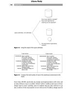
found in the customer subject area. Another interesting aspect of the customer
subject area is that it may reside on different media, as shown in Figure 2.8.
There is nothing to say that a physical table must reside on disk, even if it
relates to other data that does reside on a disk.
Figure 2.8 shows that some of the related subject area data resides on direct
access storage device (DASD) and some resides on magnetic tape. One impli-
cation of data residing on different media is that there may be more than one
DBMS managing the data in a warehouse or that some data may not be man-
aged by a DBMS at all. Just because data resides on magnetic tape or some stor-
age media other than disk storage does not mean that the data is not a part of
the data warehouse.
Data that has a high probability of access and a low volume of storage resides
on a medium that is fast and relatively expensive. Data that has a low probabil-
ity of access and is bulky resides on a medium that is cheaper and slower to
access. Usually (but not always) data that is older has a lower probability of
access. As a rule, the older data resides on a medium other than disk storage.
DASD and magnetic tape are the two most popular media on which to store
data in a data warehouse. But they are not the only media; two others that
should not be overlooked are fiche and optical disk. Fiche is good for storing
The Data Warehouse Environment
39

customer
customer activity
detail 1990–1991
customer activity
detail 1987–1989
base customer
data 1988–1990
base customer
data 1985–1987
customer activity
1986–1989
Figure 2.8 The subject area may contain data on different media in the data ware-
house.
Uttama Reddy
detailed records that never have to be reproduced in an electronic medium
again. Legal records are often stored on fiche for an indefinite period of time.
Optical disk storage is especially good for data warehouse storage because it is
cheap, relatively fast, and able to hold a mass of data. Another reason why opti-
cal disk is useful is that data warehouse data, once written, is seldom, if ever,
updated. This last characteristic makes optical disk storage a very desirable
choice for data warehouses.
Another interesting aspect of the files (shown in Figure 2.8) is that there is both
a level of summary and a level of detail for the same data. Activity by month is
summarized. The detail that supports activity by month is stored at the mag-
netic tape level of data. This is a form of a “shift in granularity,” which will be
discussed later.
When data is organized around the subject-in this case, the customer—each key
has an element of time, as shown in Figure 2.9.
CHAPTER 2
40

customer ID
month
number of transactions
average tx amount
tx high
tx low
txs cancelled

customer ID
activity date
amount
location
for item
invoice no
clerk ID
order no

customer ID
activity date
amount
location
order no
line item no
sales amount
invoice no
deliver to

customer ID
from data
to date

name
address
credit rating
employer
dob
sex

customer ID
from date
to date
name
address
phone
dob
sex

Figure 2.9 Each table in the data warehouse has an element of time as a part of the
key structure, usually the lower part.
Uttama Reddy
Some tables are organized on a from-date-to-date basis. This is called a contin-
uous organization of data. Other tables are organized on a cumulative monthly
basis, and others on an individual date of record or activity basis. But all
records have some form of date attached to the key, usually the lower part of
the key.
Day 1-Day n Phenomenon
Data warehouses are not built all at once. Instead, they are designed and popu-
lated a step at a time, and as such are evolutionary, not revolutionary. The costs
of building a data warehouse all at once, the resources required, and the dis-
ruption to the environment all dictate that the data warehouse be built in an
orderly iterative, step-at-a-time fashion. The “big bang” approach to data ware-

house development is simply an invitation to disaster and is never an appropri-
ate alternative.
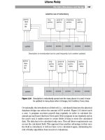
Figure 2.10 shows the typical process of building a data warehouse. On day 1
there is a polyglot of legacy systems essentially doing operational, transactional
processing. On day 2, the first few tables of the first subject area of the data
warehouse are populated. At this point, a certain amount of curiosity is raised,
and the users start to discover data warehouses and analytical processing.
On day 3, more of the data warehouse is populated, and with the population of
more data comes more users. Once users find there is an integrated source of
data that is easy to get to and has a historical basis designed for looking at data
over time, there is more than curiosity. At about this time, the serious DSS ana-
lyst becomes attracted to the data warehouse.
On day 4, as more of the warehouse becomes populated, some of the data that
had resided in the operational environment becomes properly placed in the
data warehouse. And the data warehouse is now discovered as a source for
doing analytical processing. All sorts of DSS applications spring up. Indeed, so
many users and so many requests for processing, coupled with a rather large
volume of data that now resides in the warehouse, appear that some users are
put off by the effort required to get to the data warehouse. The competition to
get at the warehouse becomes an obstacle to its usage.
On day 5, departmental databases (data mart or OLAP) start to blossom.
Departments find that it is cheaper and easier to get their processing done by
bringing data from the data warehouse into their own departmental processing
environment. As data goes to the departmental level, a few DSS analysts are
attracted.
The Data Warehouse Environment
41
Uttama Reddy
CHAPTER 2
42

existing systems
day 2
1st subject area
data warehouse
existing systems
day 3
more subjects
The warehouse
starts to become
fully populated
and access to it
arises as an issue.
existing systems
day 4
More data is
poured into the
data warehouse
and much
attention now
focuses on
departmental data
since it is easier to
get to.
operational
day 6
operational
day
n
day 1
existing systems

The warehouse
grows and the
departmental
level of processing
starts to blossom.
existing systems
day 5
Figure 2.10 Day 1-day n phenomenon.
Uttama Reddy
On day 6, the land rush to departmental systems takes place. It is cheaper,
faster, and easier to get departmental data than it is to get data from the data
warehouse. Soon end users are weaned from the detail of data warehouse to
departmental processing.
On day n, the architecture is fully developed. All that is left of the original set of
production systems is operational processing. The warehouse is full of data.
There are a few direct users of the data warehouse. There are a lot of depart-
mental databases. Most of the DSS analytical processing occurs at the depart-
mental level because it is easier and cheaper to get the data needed for
processing there.
Of course, evolution from day 1 to day n takes a long time. The evolution does
not happen in a matter of days. Several years is the norm. During the process of
moving from day 1 to day n the DSS environment is up and functional.
Note that the spider web seems to have reappeared in a larger, more grandiose
form. Such is not the case at all, although the explanation is rather complex.
Refer to “The Cabinet Effect,” in the May 1991 edition of Data Base Program-
ming Design, for an in-depth explanation of why the architected environment
is not merely a recreation of the spider web environment.
The day 1-day n phenomenon described here is the ideal way to get to the data
warehouse. There are many other paths. One such path is through the building
of data marts first. This path is short sighted and leads to a great deal of waste.

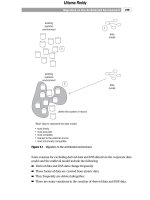
Granularity
The single most important aspect of design of a data warehouse is the issue of
granularity. Indeed, the issue of granularity permeates the entire architecture
that surrounds the data warehouse environment. Granularity refers to the level
of detail or summarization of the units of data in the data warehouse. The more
detail there is, the lower the level of granularity. The less detail there is, the
higher the level of granularity.
For example, a simple transaction would be at a low level of granularity. A sum-
mary of all transactions for the month would be at a high level of granularity.
Granularity of data has always been a major design issue. In early operational
systems, granularity was taken for granted. When detailed data is being
updated, it is almost a given that data be stored at the lowest level of granular-
ity. In the data warehouse environment, though, granularity is not assumed. Fig-
ure 2.11 illustrates the issues of granularity.
The Data Warehouse Environment
43
Uttama Reddy
Granularity is the major design issue in the data warehouse environment
because it profoundly affects the volume of data that resides in the data ware-
house and the type of query that can be answered. The volume of data in a ware-
house is traded off against the level of detail of a query.
In almost all cases, data comes into the data warehouse at too high a level of
granularity. This means that the developer must spend a lot of resources break-
ing the data apart. Occasionally, though, data enters the warehouse at too low a
level of granularity. An example of data at too low a level of granularity is the
Web log data generated by the Web-based ebusiness environment. Web log
clickstream data must be edited, filtered, and summarized before its granular-
ity is fit for the data warehouse environment.
CHAPTER 2
44

granularity—
the level of detail
high level of detail—
low level of granularity
EXAMPLE:
the details of every
phone call made by a
customer for a month
low level of detail—
high level of granularity
EXAMPLE:
the summary of phone
calls made by a
customer for a month
partitioning of data
• the splitting of data into small units
• done at the application level or the
DBMS level
easy to manage
difficult to manage
(
a
)
(
b
)
Figure 2.11 Major design issues of the data warehouse: granularity, partitioning, and
proper design.
Uttama Reddy
The Benefits of Granularity

Many organizations are surprised to find that data warehousing provides an
invaluable foundation for many different types of DSS processing. Organiza-
tions may build a data warehouse for one purpose, but they discover that it can
be used for many other kinds of DSS processing. Although infrastructure for
the data warehouse is expensive and difficult to build, it has to be built only
once. After the data warehouse has been properly constructed, it provides the
organization with a foundation that is extremely flexible and reusable.
The granular data found in the data warehouse is the key to reusability, because
it can be used by many people in different ways. For example, within a corpo-
ration, the same data might be used to satisfy the needs of marketing, sales, and
accounting. All three departments look at the basic same data. Marketing may
want to see sales on a monthly basis by geographic district, sales may want to
see sales by salesperson by sales district on a weekly basis, and finance may
want to see recognizable revenue on a quarterly basis by product line. All of
these types of information are closely related, yet slightly different. With a data
warehouse, the different organizations are able to look at the data as they wish
to see it.
Looking at the data in different ways is only one advantage of having a solid
foundation. A related benefit is the ability to reconcile data, if needed. Once
there is a single foundation on which everyone relies, if there is a need to
explain a discrepancy in analyses between two or more departments, then rec-
onciliation is relatively simple.
Another related benefit is flexibility. Suppose that marketing wishes to alter
how it looks at data. Having a foundation in place allows this to be accom-
plished easily.
Another benefit of granular data is that it contains a history of activities and
events across the corporation. And the level of granularity is detailed enough
that the data can be reshaped across the corporation for many different needs.
But perhaps the largest benefit of a data warehouse foundation is that future
unknown requirements can be accommodated. Suppose there is a new require-

ment to look at data, or the state legislature passes a new law, or OPEC changes
its rules for oil allocation, or the stock market crashes. There is a constant
stream of new requirements for information because change is inevitable. With
the data warehouse in place, the corporation can easily respond to change.
When a new requirement arises and there is a need for information, the data
warehouse is already available for analysis, and the organization is prepared to
handle the new requirements.
The Data Warehouse Environment
45
Uttama Reddy