Building the Data Warehouse Third Edition phần 3 doc

Data Warehouse: The Standards Manual
The data warehouse is relevant to many people-managers, DSS analysts, devel-
opers, planners, and so forth. In most organizations, the data warehouse is new.
Accordingly, there should be an official organizational explanation and descrip-
tion of what is in the data warehouse and how the data warehouse can be used.
Calling the explanation of what is inside the data warehouse a “standards man-
ual” is probably deadly. Standards manuals have a dreary connotation and are
famous for being ignored and gathering dust. Yet, some form of internal publi-
cation is a necessary and worthwhile endeavor.
The kinds of things the publication (whatever it is called!) should contain are
the following:
■■
A description of what a data warehouse is
■■
A description of source systems feeding the warehouse
■■
How to use the data warehouse
■■
How to get help if there is a problem
■■
Who is responsible for what
■■
The migration plan for the warehouse
■■
How warehouse data relates to operational data
■■
How to use warehouse data for DSS
■■
When not to add data to the warehouse
■■
What kind of data is not in the warehouse

■■
A guide to the meta data that is available
■■
What the system of record is
Auditing and the Data Warehouse
An interesting issue that arises with data warehouses is whether auditing can
be or should be done from them. Auditing can be done from the data ware-
house. In the past there have been a few examples of detailed audits being per-
formed there. But there are many reasons why auditing—even if it can be done
from the data warehouse—should not be done from there. The primary reasons
for not doing so are the following:
■■
Data that otherwise would not find its way into the warehouse suddenly
has to be there.
CHAPTER 2
64
Uttama Reddy
■■
The timing of data entry into the warehouse changes dramatically when
auditing capability is required.
■■
The backup and recovery restrictions for the data warehouse change dras-
tically when auditing capability is required.
■■
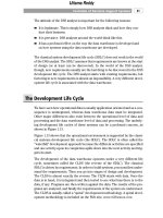
Auditing data at the warehouse forces the granularity of data in the ware-
house to be at the very lowest level.
In short, it is possible to audit from the data warehouse environment, but due
to the complications involved, it makes much more sense to audit elsewhere.
Cost Justification
Cost justification for the data warehouse is normally not done on an a priori,

return-on-investment (ROI) basis. To do such an analysis, the benefits must be
known prior to building the data warehouse.
In most cases, the real benefits of the data warehouse are not known or even
anticipated before construction begins because the warehouse is used differ-
ently than other data and systems built by information systems. Unlike most
information processing, the data warehouse exists in a realm of “Give me what
I say I want, then I can tell you what I really want.” The DSS analyst really can-
not determine the possibilities and potentials of the data warehouse, nor how
and why it will be used, until the first iteration of the data warehouse is avail-
able. The analyst operates in a mode of discovery, which cannot commence
until the data warehouse is running in its first iteration. Only then can the DSS
analyst start to unlock the potential of DSS processing.
For this reason, classical ROI techniques simply do not apply to the data ware-
house environment. Fortunately, data warehouses are built incrementally. The
first iteration can be done quickly and for a relatively small amount of money.
Once the first portion of the data warehouse is built and populated, the analyst
can start to explore the possibilities. It is at this point that the analyst can start
to justify the development costs of the warehouse.
As a rule of thumb, the first iteration of the data warehouse should be small
enough to be built and large enough to be meaningful. Therefore, the data ware-
house is best built a small iteration at a time. There should be a direct feedback
loop between the warehouse developer and the DSS analyst, in which they are
constantly modifying the existing warehouse data and adding other data to the
warehouse. And the first iteration should be done quickly. It is said that the ini-
tial data warehouse design is a success if it is 50 percent accurate.
The Data Warehouse Environment
65
Uttama Reddy
Typically, the initial data warehouse focuses on one of these functional areas:
■■

Finance
■■
Marketing
■■
Sales
Occasionally, the data warehouse’s first functional area will focus on one of
these areas:
■■
Engineering/manufacturing
■■
Actuarial interests
Justifying Your Data Warehouse
There is no getting around the fact that data warehouses cost money. Data,
processors, communications, software, tools, and so forth all cost money. In
fact, the volumes of data that aggregate and collect in the data warehouse go
well beyond anything the corporation has ever seen. The level of detail and the
history of that detail all add up to a large amount of money.
In almost every other aspect of information technology, the major investment
for a system lies in creating, installing, and establishing the system. The ongo-
ing maintenance costs for a system are miniscule compared to the initial costs.
However, establishing the initial infrastructure of the data warehouse is not the
most significant cost—the ongoing maintenance costs far outweigh the initial
infrastructure costs. There are several good reasons why the costs of a data
warehouse are significantly different from the cost of a standard system:
■■
The truly enormous volume of data that enters the data warehouse.
■■
The cost of maintaining the interface between the data warehouse and the
operational sources. If the organization has chosen an extract/transfer/load
(ETL) tool, then these costs are mitigated over time; if an organization has

chosen to build the interface manually, then the costs of maintenance sky-
rocket.
■■
The fact that a data warehouse is never done. Even after the initial few
iterations of the data warehouse are successfully completed, adding more
subject areas to the data warehouse is an ongoing need.
Cost of Running Reports
How does an organization justify the costs of a data warehouse before the data
warehouse is built? There are many approaches. We will discuss one in depth
here, but be advised that there are many other ways to justify a data warehouse.
CHAPTER 2
66
Uttama Reddy
We chose this approach because it is simple and because it applies to every
organization. When the justification is presented properly, it is very difficult to
deny the powerful cost justifications for a data warehouse. It is an argument
that technicians and non-technicians alike can appreciate and understand.
Data warehousing lowers the cost of information by approximately two orders
of magnitude. This means that with a data warehouse an organization can
access a piece of information for $100; an organization that does not have a data
warehouse can access the same unit of information for $10,000.
How do you show that data warehousing greatly lowers the cost of information?
First, use a report. This doesn’t necessarily need to be an actual report. It can be
a screen, a report, a spreadsheet, or some form of analytics that demonstrates
the need for information in the corporation. Second, you should look at your
legacy environment, which includes single or multiple applications, old and new
applications. The applications may be Enterprise Resource Planning (ERP)
applications, non-ERP applications, online applications, or offline applications.
Now consider two companies, company A and company B. The companies are
identical in respect to their legacy applications and their need for information.

The only difference between the two is that company B has a data warehouse
from which to do reporting and company A does not.
Company A looks to its legacy applications to gather information. This task
includes the following:
■■
Finding the data needed for the report
■■
Accessing the data
■■
Integrating the data
■■
Merging the data
■■
Building the report
Finding the data can be no small task. In many cases, the legacy systems are not
documented. There is a time-honored saying: Real programmers don’t do docu-
mentation. This will come back to haunt organizations, as there simply is no
easy way to go back and find out what data is in the old legacy systems and
what processing has occurred there.
Accessing the data is even more difficult. Some of the legacy data is in Infor-
mation Management System (IMS), some in Model 204, some in Adabas. And
there is no IMS, Model 204, and Adabas technology expertise around anymore.
The technology that houses the legacy environment is a mystery. And even if
the legacy environment can be accessed, the computer operations department
stands in the way because it does not want anything in the way of the online
window of processing.
The Data Warehouse Environment
67
Uttama Reddy
If the data can be found and accessed, it then needs to be integrated. Reports

typically need information from multiple sources. The problem is that those
sources were never designed to be run together. A customer in one system is
not a customer in another system, a transaction in one system is different from
a transaction in another system, and so forth. A tremendous amount of conver-
sion, reformatting, interpretation, and the like must go on in order to integrate
data from multiple systems.
Merging the data is easy in some cases. But in the case of large amounts of data
or in the case of data coming from multiple sources, the merger of data can be
quite an operation.
Finally, the report is built.
How long does this process take for company A? How much does it cost?
Depending on the information that is needed and depending on the size and
state of the legacy systems environment, it may take a considerable amount of
time and a high cost to get the information. The typical cost ranges from
$25,000 to $1 million. The typical length of time to access data is anywhere from
1 to 12 months.
Now suppose that an company B has built a data warehouse. The typical cost
here ranges from $500 to $10,000. The typical length of time to access data is
one hour to a half day. We see that company B’s costs and time investment for
retrieving information are much lower. The cost differential between company
A and company B forms the basis of the cost justification for a data warehouse.
Data warehousing greatly lowers the cost of information and accelerates the
time required to get the information.
Cost of Building the Data Warehouse
The astute observer will ask, what about the cost of building the data ware-
house? Figure 2.26 shows that in order to generate a single report for company
B, it is still necessary to find, access, integrate, and merge the data. These are
the same initial steps taken to build a single report for company A, so there are
no real savings found in building a data warehouse. Actually, building a data
warehouse to run one report is a costly waste of time and money.

But no corporation in the world operates from a single report. Different divi-
sions of even the simplest, smallest corporation look at data differently.
Accounting looks at data one way; marketing looks at data another way; sales
looks at data yet another way; and management looks at data in even another
way. In this scenario, the cost of building the data warehouse is worthwhile. It
is a one-time cost that liberates the information found in the data warehouse.
Whereas each report company A needs is both costly and time-consuming, com-
CHAPTER 2
68
TEAMFLY

Team-Fly
®

Uttama Reddy
pany B uses the one-time cost of building the data warehouse to generate mul-
tiple reports (see Figure 2.27).
But that expense is a one-time expense, for the most part. (At least the initial
establishment of the data warehouse is a one-time expense.) Figure 2.27 shows
that indeed data warehousing greatly lowers the cost of information and greatly
accelerates the rate at which information can be retrieved.
Would company A actually even pay to generate individual reports? Probably
not. Perhaps it would pay the price for information the first few times. When it
realizes that it cannot afford to pay the price for every report, it simply stops
creating reports. The end user has the attitude, “I know the information is in my
corporation, but I just can’t get to it.” The result of the high costs of getting
information and the length of time required is such that end users are frustrated
and are unhappy with their IT organization for not being able to deliver
information.
Data Homogeneity/Heterogeneity
At first glance, it may appear that the data found in the data warehouse is homo-
geneous in the sense that all of the types of records are the same. In truth, data
in the data warehouse is very heterogeneous. The data found in the data ware-
house is divided into major subdivisions called subject areas. Figure 2.28 shows
that a data warehouse has subject areas of product, customer, vendor, and
transaction.
The first division of data inside a data warehouse is along the lines of the major
subjects of the corporation. But with each subject area there are further subdi-

visions. Data within a subject area is divided into tables. Figure 2.29 shows this
division of data into tables for the subject area product.
The Data Warehouse Environment
69
5 - build the report
1 - find the data
2 - access the data
3 - integrate the data
4 - merge the data
legacy applications
data warehouse
report
Figure 2.26 Where the costs and the activities are when a data warehouse is built.
Uttama Reddy
CHAPTER 2
70
$1,000,000
$500,000
$2,000,000
$2,500,000
$1,000,000
$250
$10,000
$1,000
$2,000
$3,000
$2,000,000
company B
company A
Figure 2.27 Multiple reports make the cost of the data warehouse worthwhile.

product
customer
transaction
vendor
Figure 2.28 The data in the different parts of the data warehouse are grouped by
subject area.
Uttama Reddy
Figure 2.29 shows that there are five tables that make up the subject area inside
the data warehouse. Each of the tables has its own data, and there is a common
thread for each of the tables in the subject area. That common thread is the
key/foreign key data element—product.
Within the physical tables that make up a subject area there are further subdi-
visions. These subdivisions are created by different occurrences of data values.
For example, inside the product shipping table, there are January shipments,
February shipments, March shipments, and so forth.
The data in the data warehouse then is subdivided by the following criteria:
■■
Subject area
■■
Table
■■
Occurrences of data within table
This organization of data within a data warehouse makes the data easily acces-
sible and understandable for all the different components of the architecture
that must build on the data found there. The result is that the data warehouse,
with its granular data, serves as a basis for many different components, as seen
in Figure 2.30.
The simple yet elegant organization of data within the data warehouse environ-
ment seen in Figure 2.30 makes data accessible in many different ways for
many different purposes.

The Data Warehouse Environment
71
product
product
date
location




order
product
date




vendor
product
description





product
ship date
ship amount

product
bom number
bom description



Figure 2.29 Within the product subject area there are different types of tables, but each
table has a common product identifier as part of the key.
Uttama Reddy
Purging Warehouse Data
Data does not just eternally pour into a data warehouse. It has its own life cycle
within the warehouse as well. At some point in time, data is purged from the
warehouse. The issue of purging data is one of the fundamental design issues
that must not escape the data warehouse designer.
In some senses, data is not purged from the warehouse at all. It is simply rolled
up to higher levels of summary. There are several ways in which data is purged
or the detail of data is transformed, including the following:
CHAPTER 2
72
Fig 2.30 The data warehouse sits at the center of a large framework.
Uttama Reddy
■■
Data is added to a rolling summary file where detail is lost.
■■
Data is transferred to a bulk storage medium from a high-performance
medium such as DASD.
■■
Data is actually purged from the system.
■■
Data is transferred from one level of the architecture to another, such as

from the operational level to the data warehouse level.
There are, then, a variety of ways in which data is purged or otherwise trans-
formed inside the data warehouse environment. The life cycle of data—includ-
ing its purge or final archival dissemination—should be an active part of the
design process for the data warehouse.
Reporting and the Architected Environment
It is a temptation to say that once the data warehouse has been constructed all
reporting and informational processing will be done from there. That is simply
not the case. There is a legitimate class of report processing that rightfully
belongs in the domain of operational systems. Figure 2.31 shows where the dif-
ferent styles of processing should be located.
The Data Warehouse Environment
73
operational
operational reporting
• the line item is of the essence; the
summary is of little or no
importance once used
• of interest to the clerical community
data warehouse reporting
• the line item is of little or no use
once used; the summary or other
calculation is of primary importance
• of interest to the managerial
community
data warehouse
Figure 2.31 The differences between the two types of reporting.
Uttama Reddy
Figure 2.31 shows that operational reporting is for the clerical level and focuses
primarily on the line item. Data warehouse or informational processing focuses

on management and contains summary or otherwise calculated information. In
the data warehouse style of reporting, little use is made of line-item, detailed
information, once the basic calculation of data is made.
As an example of the differences between operational reporting and DSS
reporting, consider a bank. Every day before going home a teller must balance
the cash in his or her window. This means that the teller takes the starting
amount of cash, tallies all the day’s transactions, and determines what the day’s
ending cash balance should be. In order to do this, the teller needs a report of
all the day’s transactions. This is a form of operational reporting.
Now consider the bank vice president who is trying to determine how many
new ATMs to place in a newly developed shopping center. The banking vice
president looks at a whole host of information, some of which comes from
within the bank and some of which comes from outside the bank. The bank vice
president is making a long-term, strategic decision and uses classical DSS infor-
mation for his or her decision.
There is then a real difference between operational reporting and DSS report-
ing. Operational reporting should always be done within the confines of the
operational environment.
The Operational Window of Opportunity
In its broadest sense, archival represents anything older than right now. Thus,
the loaf of bread that I bought 30 seconds ago is archival information. The only
thing that is not archival is information that is current.
The foundation of DSS processing—the data warehouse—contains nothing but
archival information, most of it at least 24 hours old. But archival data is found
elsewhere throughout the architected environment. In particular, some limited
amounts of archival data are also found in the operational environment.
In the data warehouse it is normal to have a vast amount of archival data—from
5 to 10 years of data is common. Because of the wide time horizon of archival
data, the data warehouse contains a massive amount of data. The time horizon
of archival data found in the operational environment—the “operational win-

dow” of data—is not nearly as long. It can be anywhere from 1 week to 2 years.
The time horizon of archival data in the operational environment is not the only
difference between archival data in the data warehouse and in the operational
CHAPTER 2
74
Uttama Reddy
environment. Unlike the data warehouse, the operational environment’s
archival data is nonvoluminous and has a high probability of access.
In order to understand the role of fresh, nonvoluminous, high-probability-of-
access archival data in the operational environment, consider the way a bank
works. In a bank environment, the customer can reasonably expect to find
information about this month’s transactions. Did this month’s rent check clear?
When was a paycheck deposited? What was the low balance for the month? Did
the bank take out money for the electricity bill last week?
The operational environment of a bank, then, contains very detailed, very cur-
rent transactions (which are still archival). Is it reasonable to expect the bank
to tell the customer whether a check was made out to the grocery store 5 years
ago or whether a check to a political campaign was cashed 10 years ago? These
transactions would hardly be in the domain of the operational systems of the
bank. These transactions very old, and so the has a very low probability of
access.
The operational window of time varies from industry to industry and even in
type of data and activity within an industry.
For example, an insurance company would have a very lengthy operational win-
dow—from 2 to 3 years. The rate of transactions in an insurance company is
very low, at least compared to other types of industries. There are relatively few
direct interactions between the customer and the insurance company. The oper-
ational window for the activities of a bank, on the other hand, is very short—
from 0 to 60 days. A bank has many direct interactions with its customers.
The operational window of a company depends on what industry the company

is in. In the case of a large company, there may be more than one operational
window, depending on the particulars of the business being conducted. For
example, in a telephone company, customer usage data may have an opera-
tional window of 30 to 60 days, while vendor/supplier activity may have a win-
dow of 2 to 3 years.
The following are some suggestions as to how the operational window of
archival data may look in different industries:
■■
Insurance—2 to 3 years
■■
Bank trust processing—2 to 5 years
■■
Telephone customer usage—30 to 60 days
■■
Supplier/vendor activity—2 to 3 years
■■
Retail banking customer account activity—30 days
■■
Vendor activity—1 year
■■
Loans—2 to 5 years
The Data Warehouse Environment
75
Uttama Reddy
■■
Retailing SKU activity—1 to 14 days
■■
Vendor activity—1 week to 1 month
■■
Airlines flight seat activity— 30 to 90 days

■■
Vendor/supplier activity—1 to 2 years
■■
Public utility customer utilization—60 to 90 days
■■
Supplier activity—1 to 5 years
The length of the operational window is very important to the DSS analyst
because it determines where the analyst goes to do different kinds of analysis
and what kinds of analysis can be done. For example, the DSS analyst can do
individual-item analysis on data found within the operational window, but can-
not do massive trend analysis over a lengthy period of time. Data within the
operational window is geared to efficient individual access. Only when the data
passes out of the operational window is it geared to mass data storage and
access.
On the other hand, the DSS analyst can do sweeping trend analysis on data
found outside the operational window. Data out there can be accessed and
processed en masse, whereas access to any one individual unit of data is not
optimal.
Incorrect Data in the Data Warehouse
The architect needs to know what to do about incorrect data in the data ware-
house. The first assumption is that incorrect data arrives in the data warehouse
on an exception basis. If data is being incorrectly entered in the data warehouse
on a wholesale basis, then it is incumbent on the architect to find the offending
ETL program and make adjustments. Occasionally, even with the best of ETL
processing, a few pieces of incorrect data enter the data warehouse environ-
ment. How should the architect handle incorrect data in the data warehouse?
There are at least three options. Each approach has its own strengths and
weaknesses, and none are absolutely right or wrong. Instead, under some cir-
cumstances one choice is better than another.
For example, suppose that on July 1 an entry for $5,000 is made into an opera-

tional system for account ABC. On July 2 a snapshot for $5,000 is created in the
data warehouse for account ABC. Then on August 15 an error is discovered.
Instead of an entry for $5,000, the entry should have been for $750. How can the
data in the data warehouse be corrected?
CHAPTER 2
76
Uttama Reddy
■■
Choice 1: Go back into the data warehouse for July 2 and find the offend-
ing entry. Then, using update capabilities, replace the value $5,000 with the
value $750. This is a clean and neat solution when it works, but it intro-
duces new issues:
■■
The integrity of the data has been destroyed. Any report running
between July 2 and Aug 16 will not be able to be reconciled.
■■
The update must be done in the data warehouse environment.
■■
In many cases there is not a single entry that must be corrected, but
many, many entries that must be corrected.
■■
Choice 2: Enter offsetting entries. Two entries are made on August 16, one
for Ϫ$5,000 and another for ϩ$750. This is the best reflection of the most
up-to-date information in the data warehouse between July 2 and August
16. There are some drawbacks to this approach:
■■
Many entries may have to be corrected, not just one. Making a simple
adjustment may not be an easy thing to do at all.
■■
Sometimes the formula for correction is so complex that making an

adjustment cannot be done.
■■
Choice 3: Reset the account to the proper value on August 16. An entry on
August 16 reflects the balance of the account at that moment regardless of
any past activity. An entry would be made for $750 on August 16. But this
approach has its own drawbacks:
■■
The ability to simply reset an account as of one moment in time requires
application and procedural conventions.
■■
Such a resetting of values does not accurately account for the error that
has been made.
Choice 3 is what likely happens when you cannot balance your checking
account at the end of the month. Instead of trying to find out what the bank has
done, you simply take the bank’s word for it and reset the account balance.
There are then at least three ways to handle incorrect data as it enters the data
warehouse. Depending on the circumstances, one of the approaches will yield
better results than another approach.
Summary
The two most important design decisions that can be made concern the granu-
larity of data and the partitioning of data. For most organizations, a dual level
The Data Warehouse Environment
77
Uttama Reddy
of granularity makes the most sense. Partitioning of data breaks it down into
small physical units. As a rule, partitioning is done at the application level
rather than at the system level.
Data warehouse development is best done iteratively. First one part of the data
warehouse is constructed, then another part of the warehouse is constructed. It
is never appropriate to develop the data warehouse under the “big bang”

approach. One reason is that the end user of the warehouse operates in a dis-
covery mode, so only after the warehouse’s first iteration is built can the devel-
oper tell what is really needed in the warehouse.
The granularity of the data residing inside the data warehouse is of the utmost
importance. A very low level of granularity creates too much data, and the sys-
tem is overwhelmed by the volumes of data. A very high level of granularity is
efficient to process but precludes many kinds of analyses that need detail. In
addition, the granularity of the data warehouse needs to be chosen in an aware-
ness of the different architectural components that will feed off the data ware-
house.
Surprisingly, many design alternatives can be used to handle the issue of gran-
ularity. One approach is to build a multitiered data warehouse with dual levels
of granularity that serve different types of queries and analysis. Another
approach is to create a living sample database where statistical processing can
be done very efficiently from a living sample database.
Partitioning a data warehouse is very important for a variety of reasons. When
data is partitioned it can be managed in separate, small, discrete units. This
means that loading the data into the data warehouse will be simplified, building
indexes will be streamlined, archiving data will be easy, and so forth. There are
at least two ways to partition data—at the DBMS/operating system level and at
the application level. Each approach to partitioning has its own set of advan-
tages and disadvantages.
Each unit of data in the data warehouse environment has a moment associated
with it. In some cases, the moment in time appears as a snapshot on every
record. In other cases, the moment in time is applied to an entire table. Data is
often summarized by day, month, or quarter. In addition, data is created in a
continuous manner. The internal time structuring of data is accomplished in
many ways.
Auditing can be done from a data warehouse, but auditing should not be done
from a data warehouse. Instead, auditing is best done in the detailed opera-

tional transaction-oriented environment. When auditing is done in the data
warehouse, data that would not otherwise be included is found there, the tim-
ing of the update into the data warehouse becomes an issue, and the level of
CHAPTER 2
78
TEAMFLY

Team-Fly

®

Uttama Reddy
granularity in the data warehouse is mandated by the need for auditing, which
may not be the level of granularity needed for other processing.
A normal part of the data warehouse life cycle is that of purging data. Often,
developers neglect to include purging as a part of the specification of design.
The result is a warehouse that grows eternally, which, of course, is an impossi-
bility.
The Data Warehouse Environment
79
Uttama Reddy
Uttama Reddy
The Data Warehouse
and Design
CHAPTER
3
T
here are two major components to building a data warehouse: the design of
the interface from operational systems and the design of the data warehouse
itself. Yet, “design” is not entirely accurate because it suggests planning ele-
ments out in advance. The requirements for the data warehouse cannot be
known until it is partially populated and in use and design approaches that
have worked in the past will not necessarily suffice in subsequent data ware-
houses. Data warehouses are constructed in a heuristic manner, where one
phase of development depends entirely on the results attained in the previous
phase. First, one portion of data is populated. It is then used and scrutinized by
the DSS analyst. Next, based on feedback from the end user, the data is modi-
fied and/or other data is added. Then another portion of the data warehouse is
built, and so forth.This feedback loop continues throughout the entire life of

the data warehouse.
Therefore, data warehouses cannot be designed the same way as the classical
requirements-driven system. On the other hand, anticipating requirements is
still important. Reality lies somewhere in between.
NOTE
A data warehouse design methodology that parallels this chapter can be found—for
free—on www.billinmon.com. The methodology is iterative and all of the required
design steps are greatly detailed.
81
Uttama Reddy
Beginning with Operational Data
At the outset, operational transaction-oriented data is locked up in existing
legacy systems. Though tempting to think that creating the data warehouse
involves only extracting operational data and entering it into the warehouse,
nothing could be further from the truth. Merely pulling data out of the legacy
environment and placing it in the data warehouse achieves very little of the
potential of data warehousing.
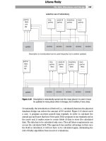
Figure 3.1 shows a simplification of how data is transferred from the existing
legacy systems environment to the data warehouse. We see here that multiple
applications contribute to the data warehouse.
Figure 3.1 is overly simplistic for many reasons. Most importantly, it does not
take into account that the data in the operational environment is unintegrated.
Figure 3.2 shows the lack of integration in a typical existing systems environ-
ment. Pulling the data into the data warehouse without integrating it is a grave
mistake.
When the existing applications were constructed, no thought was given to pos-
sible future integration. Each application had its own set of unique and private
requirements. It is no surprise, then, that some of the same data exists in vari-
ous places with different names, some data is labeled the same way in different
places, some data is all in the same place with the same name but reflects a dif-

ferent measurement, and so on. Extracting data from many places and inte-
grating it into a unified picture is a complex problem.
CHAPTER 3
82
data
warehouse
existing
applications
Figure 3.1 Moving from the operational to the data warehouse environment is not as
simple as mere extraction.
Uttama Reddy
This lack of integration is the extract programmer’s nightmare. As illustrated in
Figure 3.3, countless details must be programmed and reconciled just to bring
the data properly from the operational environment.
One simple example of lack of integration is data that is not encoded consis-
tently, as shown by the encoding of gender. In one application, gender is
encoded as m/f. In another, it is encoded as 0/1. In yet another it is encoded as
x/y. Of course, it doesn’t matter how gender is encoded as long as it is done con-
sistently. As data passes to the data warehouse, the applications’ different val-
ues must be correctly deciphered and recoded with the proper value.
As another example, consider four applications that have the same field-
pipeline. The pipeline field is measured differently in each application. In one
application, pipeline is measured in inches, in another in centimeters, and so
forth. It does not matter how pipeline is measured in the data warehouse, as
long as it is measured consistently. As each application passes its data to the
warehouse, the measurement of pipeline is converted into a single consistent
corporate measurement.
Field transformation is another integration issue. Say that the same field exists
in four applications under four different names. To transform the data to the
data warehouse properly, a mapping from the different source fields to the data

warehouse fields must occur.
Yet another issue is that legacy data exists in many different formats under
many different DBMSs. Some legacy data is under IMS, some legacy data is
under DB2, and still other legacy data is under VSAM. But all of these technolo-
gies must have the data they protect brought forward into a single technology.
Such a translation of technology is not always straightforward.
The Data Warehouse and Design
83
savings DDA loans trust
same data,
different name
different data,
same name
data found here,
nowhere else
different keys,
same data
Figure 3.2 Data across the different applications is severely unintegrated.
Uttama Reddy
These simple examples hardly scratch the surface of integration, and they are
not complex in themselves. But when they are multiplied by the thousands of
existing systems and files, compounded by the fact that documentation is usu-
ally out-of-date or nonexistent, the issue of integration becomes burdensome.
But integration of existing legacy systems is not the only difficulty in the trans-
formation of data from the operational, existing systems environment to the
data warehouse environment. Another major problem is the efficiency of
accessing existing systems data. How does the program that scans existing sys-
tems know whether a file has been scanned previously? The existing systems
environment holds tons of data, and attempting to scan all of it every time a
data warehouse load needs to be done is wasteful and unrealistic.

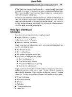
Three types of loads are made into the data warehouse from the operational
environment:
■■
Archival data
■■
Data currently contained in the operational environment
■■
Ongoing changes to the data warehouse environment from the changes
(updates) that have occurred in the operational environment since the last
refresh
As a rule, loading archival data from the legacy environment as the data ware-
house is first loaded presents a minimal challenge for two reasons. First, it
CHAPTER 3
84
appl A –balance
appl B –bal
appl C –currbal
appl D –balcurr
field transformation
appl A –pipeline–cm
appl B –pipeline–in
appl C –pipeline–mcf
appl D –pipeline–yds
unit of measure transformation
appl A –m,f
appl B –1,0
appl C –x,y
appl D –male, female
encoding transformation
m,f

data warehouse
cm
data warehouse
bal
data warehouse
Figure 3.3 To properly move data from the existing systems environment to the data
warehouse environment, it must be integrated.
Uttama Reddy
often is not done at all. Organizations find the use of old data not cost-effective
in many environments. Second, even when archival data is loaded, it is a one-
time-only event.
Loading current, nonarchival data from the existing operational environment
likewise presents a minimal challenge because it needs to be done only once.
Usually, the existing systems environment can be downloaded to a sequential
file, and the sequential file can be downloaded into the warehouse with no dis-
ruption to the online environment. Although system resources are required,
because the process is done only once, the event is minimally disruptive.
Loading data on an ongoing basis—as changes are made to the operational
environment—presents the largest challenge to the data architect. Efficiently
trapping those ongoing daily changes and manipulating them is not easy. Scan-
ning existing files, then, is a major issue facing the data warehouse architect.
Five common techniques are used to limit the amount of operational data
scanned at the point of refreshing the data warehouse, as shown in Figure 3.4.
The first technique is to scan data that has been timestamped in the operational
environment. When an application stamps the time of the last change or update
on a record, the data warehouse scan can run quite efficiently because data
with a date other than that applicable does not have to be touched. It usually is
only by happenstance, though, that existing data has been timestamped.
The second technique to limiting the data to be scanned is to scan a “delta” file.
A delta file contains only the changes made to an application as a result of the

transactions that have run through the operational environment. With a delta
file, the scan process is very efficient because data that is not a candidate for
scanning is never touched. Not many applications, however, build delta files.
The third technique is to scan a log file or an audit file created as a by-product of
transaction processing. A log file contains essentially the same data as a delta
file; however, there are some major differences. Many times, operations protects
the log files because they are needed in the recovery process. Computer opera-
tions is not particularly thrilled to have its log file used for something other than
its primary purpose. Another difficulty with a log tape is that the internal format
is built for systems purposes, not applications purposes. A technological guru
may be needed to interface the contents of data on the log tape. Another short-
coming is that the log file usually contains much more information than that
desired by the data warehouse developer. Audit files have many of the same
shortcomings as log files. An example of the use of log files to update a data
warehouse is the Web logs created by the Web-based ebusiness environment.
The fourth technique for managing the amount of data scanned is to modify
application code. This is never a popular option, as much application code is
old and fragile.
The Data Warehouse and Design
85
Uttama Reddy
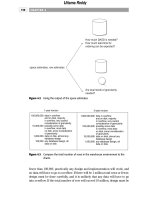
The last option (in most respects, a hideous one, mentioned primarily to con-
vince people that there must be a better way) is rubbing a “before” and an
“after” image of the operational file together. In this option, a snapshot of a
database is taken at the moment of extraction. When another extraction is per-
formed, another snapshot is taken. The two snapshots are serially compared to
each other to determine the activity that has transpired. This approach is cum-
bersome and complex, and it requires an inordinate amount of resources. It is
simply a last resort to be done when nothing else works.
Integration and performance are not the only major discrepancies that prevent

a simple extract process from being used to construct the data warehouse. A
third difficulty is that operational data must undergo a time-basis shift as it
passes into the data warehouse, as shown in Figure 3.5.
Existing operational data is almost always current-value data. Such data’s accu-
racy is valid as of the moment of access, and it can be updated. But data that
CHAPTER 3
86
existing
applications
time stamped
existing
applications
delta
file
existing
applications
log or
audit file
existing
applications
application
code
before
image
changes
to database
since last update
after
image
Figure 3.4 How do you know what source data to scan? Do you scan every record every

day? Every week?
Uttama Reddy
goes into the data warehouse cannot be updated. Instead, an element of time
must be attached to it. A major shift in the modes of processing surrounding the
data is necessary as it passes into the data warehouse from the operational
environment.
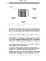
Yet another major consideration when passing data is the need to manage the
volume of data that resides in and passes into the warehouse. Data must be
condensed both at the moment of extraction and as it arrives at the warehouse.
If condensation is not done, the volume of data in the data warehouse will grow
rapidly out of control. Figure 3.6 shows a simple form of data condensation.
Data/Process Models and the
Architected Environment
Before attempting to apply conventional database design techniques, the
designer must understand the applicability and the limitations of those tech-
niques. Figure 3.7 shows the relationship among the levels of the architecture
and the disciplines of process modeling and data modeling. The process model
applies only to the operational environment. The data model applies to both the
operational environment and the data warehouse environment. Trying to use a
process or data model in the wrong place produces nothing but frustration.
The Data Warehouse and Design
87
balance taken
at end of day
a new balance created
upon successful completion
of a transaction
current value
current value
current value

current value
current value
current value
current value
daily
balance
daily
balance
daily
balance
time basis shift
tx
tx
tx
tx
tx
tx
Figure 3.5 A shift in time basis is required as data is moved over from the operational
to the data warehouse environment.
Uttama Reddy
In general there are two types of models for the information systems environ-
ment—data models and process models. Data models are discussed in depth in
the following section. For now, we will address process models. A process
model typically consists of the following (in whole or in part):
■■
Functional decomposition
■■
Context-level zero diagram
■■
Data flow diagram

■■
Structure chart
■■
State transition diagram
■■
HIPO chart
■■
Pseudocode
There are many contexts and environments in which a process model is invalu-
able—for instance, when building the data mart. However, because the process
model is requirements-based, it is not suitable for the data warehouse. The
process model assumes that a set of known processing requirements exists—a
priori—before the details of the design are established. With processes, such an
assumption can be made. But those assumptions do not hold for the data ware-
house. Many development tools, such as CASE tools, have the same orientation
and as such are not applicable to the data warehouse environment.
CHAPTER 3
88
managing volumes of data
current value
current value
tx
daily
balance
weekly
balance
monthly
balance
If the volumes of data are not
carefully managed and condensed,

the sheer volume of data that
aggregates in the data warehouse
prevents the goals of the
warehouse from being achieved.
Figure 3.6 Condensation of data is a vital factor in the managing of warehouse data.
TEAMFLY

Team-Fly

®

Uttama Reddy