Fundamentals of Electrical Drivess - Chapter 1 pptx

Chapter 1
INTRODUCTION
1.1 Why use electro-mechanical energy conversion?
Electric motors are around us everywhere. Generators in power plants are
connected to a three-phase power grid of alternating current (AC), pumps in
your heating system, refrigerator and vacuum cleaner are connected to a single
phase AC grid and switched on or off by means of a simple contactor. In cars
a direct current (DC) battery is used to provide power to the starter motor,
windshield wiper motors and other utilities. These motors run on direct current
and in most cases they are activated by a relay switch without any control.
Many applications driven by electric motors require more or less advanced
control. Lowering the speed of a fan or pump can be considered relatively
simple. Perhaps one of the most difficult ones is the dynamic positioning of a
tug in a wafer-stepper with nanometer accuracy while accelerating at several g’s.
Another challenging controlled drive is an electric crane in a harbor that needs
to be able to move an empty hook at high speed, navigate heavy loads up and
down at moderate velocities and make a soft touchdown as close as possible to
its intended final position. Other applications such as assembly robots, electric
elevators, electric motor control in hybrid vehicles, trains, streetcars, or CD-
players can, with regard to complexity, be situated somewhere in between.
Design and analysis of all electric drive systems require not only knowledge
of dynamic properties of different motor types, but also a good understanding
of the way these motors interact with power-electronic converters. These power
converters are used to control motor currents or voltages in various manners.
Compared to other drive systems such as steam engines (still used for aircraft
launch assist), hydraulic engines (famous for their extreme power per volume),
pneumatic drives (famous for their simplicity, softness and hissing sound), com-
bustion engines in vehicles or turbo-jet drives in helicopters or aircraft, electric
2 FUNDAMENTALS OF ELECTRICAL DRIVES
drive systems have a very wide field of applications thanks to some strong
points:

Large power range available: actuators and drives are used in a very wide
range of applications from wrist-watch level to machines at the multi-
megawatt level, i.e. as used in coal mines and the steel industry.
Electrical drives are capable of full torque at standstill, hence no clutches
are required.
Electrical drives can provide a very large speed range, usually gearboxes
can be omitted.
Clean operation, no oil-spills to be expected.
Safe operation possible in environments with explosive fumes (pumps in
oil-refineries).
Immediate use: electric drives can be switched on immediately.
Low service requirement: electrical drives do not require regular service as
there are very few components subject to wear, except the bearings. This
means that electrical drives have a long life expectancy, typically in excess
of twenty years.
Low no-load losses: when a drive is running idle, little power is dissipated
since no oil needs to be pumped around to keep it lubricated. Typical
efficiency levels for a drive is in the order of 85% in some cases this may
be as high as 98%. The higher the efficiency the more costly the drive
technology, in terms of initial costs.
Electric drives produce very little acoustic noise compared to combustion
engines.
Excellent control ability: electrical drives can be made to conform to precise
user requirements. This may, for example, be inrelationtorealizingacertain
shaft speed or torque level.
‘Four-quadrant operation’: Motor- and braking-mode are both possible in
forward or reverse direction, yielding four different quadrants: forward
motoring, forward braking, reverse motoring and reverse braking. Positive
speed is called forward, reverse indicates negative speed. A machine is in
motor mode when energy is transferred from the power source to the shaft

i.e. when both torque and speed have the same sign.
Introduction 3
1.1.1 Modes of operation
When a machine is in motoring mode, most of the energy is transferred from
the electrical power source to the mechanical load. Motoring mode takes place
in quadrants 1 and 3 (see figure 1.1(b). If the shaft torque and shaft speed are
in opposition then the flow of energy is reversed, in which case the drive is in
the so-called ‘braking’ mode.
(a) Motor with power supply (b) Operating modes
Figure 1.1. Motoring and braking operation
Braking comes in three ‘flavours’. The first is referred to as ‘regenera-
tive’ braking operation, where most of the mechanical energy from the load is
returned to the power source. Most drives which contain a converter (see sec-
tion 1.2) between motor and supply use a diode rectifier as a front end, hence
power can only flow from the AC power-grid to the DC-link in the drive and
not the other way around. In such converters regenerative operation is only
possible when the internal DC-link of the drive is shared with other drives that
are able to use the regenerated power immediately. Sharing a common rectifier
with many drives is economic and becoming standard practise. Furthermore,
attention is drawn to the fact that some power sources are not able to accept any
(or only a limited amount (batteries)) regenerated energy.
The second option is referred to as ‘dissipative’ braking operation where
most of the mechanical load energy is burned up in an external brake-chopper-
resistor. A brake-chopper can burn away a substantial part of the rated power
for several seconds, designed to be sufficient to stop the mechanical system in a
fast and safe fashion. One can regard such a brake-chopper as a big zener-diode
that prevents the DC-link voltage in the converter from rising too high. Brake
choppers come in all sizes, in off-shore cranes and locomotives, power levels
of several megawatts are common practise.
4 FUNDAMENTALS OF ELECTRICAL DRIVES

The third braking mode is one where mechanical power is completely re-
turned to the motor at the same time some or none electrical power is delivered,
i.e. both mechanical and electrical input power are dissipated in the motor.
Think of a permanent magnet motor being shorted, or an induction motor that
carries a DC current in its stator, acting as an eddy-current-brake.
Of coursethereare alsodisadvantageswhenusing electricaldrive technology,
a few of these are briefly outlined below.
Low torque/force density compared to combustion engines or hydraulic
systems. This is why aircraft control systems are still mostly hydraulic.
However, there is an emerging trend in this industry to use electrical drives
instead of hydraulic systems.
High complexity: A modern electrical drive encompasses a range of tech-
nologies as will become apparent in this book. This means that it requires
highly skilled personnel to repair or modify such systems.
1.2 Key components of an electrical drive system
The ‘drive’ shown in figure 1.1(a) is in fact only an electrical machine con-
nected directly to a power supply. This configuration is widely in use but one
cannot exert very much control in terms of controlling torque and/or speed.
Such drives are either on or off with rather wild starting dynamics. The drive
concept of primary interest in this book is capable of what is referred to as
‘adjustable speed’ operation [Miller, 1989] which means that the machine can
be made to operate over a wide speed range. A simplified structure of a drive
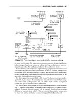
is shown in figure 1.2. A brief description of the components is given below:
Figure 1.2. Typical drive set-up
Load: This component is central to the drive in that the purpose of the
drive is to meet specific mechanical load requirements. It is emphasized
Introduction 5
that it is important to fully understand the nature of the load and the user
requirements which must be satisfied by the drive. The load component may
or may not have sensors to measure either speed, torque or shaft angle. The

sensors which can be used are largely determined by the application. The
nature of the load may be translational or rotational and the drive designer
must make a prudent choice wether to use a direct-drive with a large motor
or geared drive with a smaller but faster one. Furthermore, the nature of the
load in terms of the need for continuous or intermittent operation must be
determined.
Motor: A limited range of motor types is presently in use. Among these are
the so-called ‘classical’ machines, which have their origins at the turn of the
19th century. This classical machine set has displaced a large assortment
of ‘specialized’ machines used prior to the introduction of power electronic
converters for speed control. This classical machine set contains the DC
(Direct Current) machine, asynchronous (induction) machine, synchronous
machine and ‘variable reluctance’ machine. Of these the ‘variable reluc-
tance’ machine will not be discussed in this book. A detailed discussion
of this machine appears in the second book ‘Advanced Electrical Drives’
written by the authors of this book. An illustration of the improvements in
terms of the power to weight ratio which has been achieved over the past
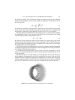
century is given in figure 1.3.
Figure 1.3. Power density of electrical machines over the past century
The term ‘motor’ refers to a machine which operates as a motor, i.e. energy
flows from the motor to the load. When the energy flows in the opposite
direction a machine is said to operate as a generator.
6 FUNDAMENTALS OF ELECTRICAL DRIVES
Converter: This unit contains a set of power electronic switches which are
used to manipulate the energy transfer between power supply and motor.
The use of switches is important given that no power is dissipated (in the
ideal case) when the switches are either open or closed. Hence, theoretically
the efficiency of such a converter is 100%, whichis important particularly for
large converters given the impossibility of absorbing large losses which usu-
ally appear in the form of heat. A large range of power electronic switches

is available to the designer to meet a wide range of applications.
Modulator: The switches within the converter are controlled by the mod-
ulator which determines which switches should be on, and for what time
interval, normally on a micro-second timescale. An example is the Pulse
Width Modulator that realizes a required pulse width at a given carrier-
frequency of a few kHz.
Controller: The controller, typically a digital signal processor (DSP), or
micro-controller contains a number of software based control loops which
control, for example, the currents in the converter and machine. In addi-
tion torque, speed and shaft angle control loops may be present within this
module. Shown in the diagram are the various sensor signals which form
the key inputs to the controller together with a number of user set-points
(not shown in the diagram). The output of the controller is a set of control
parameters which are used by the modulator.
Digital Link: This unit serves as the interface between the controller and an
external computer. With the aid of this link drive set-points and diagnostical
information can be exchanged with a remote user.
Power supply: In most cases the converter requires a DC voltage source.
The power can be obtained from a DC power source, in case one is available.
However, inmost cases theDCpowerrequirementsare met viaarectification
process, which makes use of the single or three-phase AC (referred to as the
‘grid’) power supply as provided by the utility grid.
1.3 What characterizes high performance drives?
Prior to moving to a detailed discussion of the various drive components it is
important to understand the reasons behind the ongoing development of drives.
Firstly, an observation of the drive structure (see figure 1.2) learns that the drive
has components which cover a very wide field of knowledge. For example,
moving from load to controller one needs to appreciate the nature of the load,
have a thorough understanding of the motor, comprehend the functioning of the
converter and modulator. Finally, one needs tounderstand the control principles

involved andhowtoimplement (in software)the control algorithmsintoa micro-
processor or DSP. Hence there is a need to have a detailed understanding of a
Introduction 7
very wide range of topics which is perhaps one of the most challenging aspects
of working in this field.
The development of electrical machines occurred, as was mentioned earlier,
more than a century ago. However, the step to a high performance drive took
considerably longer and is in fact still ongoing. The main reasons as to why
drive technology has improved over the last decades are briefly outlined below:
Availability of fast and reliable power semiconductor switches for the con-
verter: A range of switches is available to the user today to design and build
a wide range of converter topologies. The most commonly used switch-
ing devices for motor drives are MOSFET’s for low voltage applications,
IGBT’s for medium (kW) and higher (MW) powers. In addition GCT’s are
available for medium and high voltage applications.
Availability of fast computers for (real time) embedded control: the con-
troller needs to provide the control input to the modulator at a sampling
rate which is typically in the order of 100µs. Within that time frame the
computer needs to acquire the input data from sensors and user set-points
and apply the control algorithm in order to calculate the control outputs for
the next cycle. The presence of low cost fast micro-processors or DSP’s has
been of key importance for drive development.
Better sensors: A range of reliable and low cost sensors is available to
the user which provides accurate inputs for the controller such as LEM’s,
incremental encoders and Hall-effect sensors.
Better simulation packages: Sophisticated so-called ‘finite-element’ com-
puter aided design (CAD) packages for motor design have been instrumental
in gaining a better understanding of machines. Furthermore, they have been
and continue to be used for designing machines and for optimization pur-
poses. In terms of simulating the entire drive structure there are simulators

with graphical user interfaces, such as among others MATLAB/Simulink
R

and Caspoc, which allow the user to analyze a detailed dynamic model of
the entire system. This means that one can analyze the behaviour of such
a system under a range of conditions and explore new control techniques
without the need of actually building the entire system. This does not mean
that implementing real life systems is no longer required. The proof of the
pudding is in the eating, and only experimental validation can prove that the
supposed models are indeed valid for a real drive system.
Simulation and experiment are never exactly the same. When the models
are not able to describe the drive system under certain conditions, it might be
useful to enhance the simulation model to incorporate some of the found dif-
ferences. As engineers we should be aware of the fact that drive systems are
often closed-loop systems that are able to tolerate deviations in parameters
8 FUNDAMENTALS OF ELECTRICAL DRIVES
and unknown load torques without any problem. To paraphrase Einstein,
‘A simulation model should be as simple as possible, but no simpler’ is
the key to a successful simulation. This means that essential dynamics or
non-linearities found in the real world system, need to be implemented in
the (physics based) simulation model in order to study extreme situations
with acceptable accuracy.
The simulation model used depends on what needs to be studied. Simulating
pulse-width modulated outputs requires a very short simulation time-step,
in the order of sub-µs or so, while the overall mechanical system and the
motor’s response can be calculated at a hundred times larger time-step with
negligible loss of accuracy, as long as the power converter is regarded as a
non-switching controlled voltage source. Another extreme example is the
study of thermal effects on the motor, in that case only the average power
dissipation in terms of seconds or even minutes is of interest.

Better materials: The availability of improved magnetic, electrical and in-
sulation materials has provided the basis for efficient machines capable of
withstanding higher temperatures, thereby offering long application life and
low life cycle costs.
1.4 Notational conventions
1.4.1 Voltage and current conventions
The conventions used in this book for the voltage and current variables are
shown with the aid of figure 1.4. The diagram shows the variables voltage u and
Figure 1.4. Notation conventions used for electrical quantities
current i, which are specifically given in ‘lower case’ notation, because they
represent instantaneous values, i.e. a function of time. The ‘voltage arrows’
shown in figure 1.4 point to the negative terminal of the respective circuit.
Introduction 9
1.4.2 Mechanical conventions
The mechanical conventions used in this book are shown with the aid of
figure 1.5. The electromagnetictorque T
e
produced bythe machine corresponds
with a power output p
e
= T
e
ω
m
,whereω
m
represents the rotational speed,
otherwise known as the angular frequency. The load torque T
L
is linked to the

power delivered to the load p
L
= T
l
ω
m
. The torque difference T
e
−T
l
results
in an acceleration Jdω
m
/dt of the rotating mass with inertia J. This rotating
structure is represented as a lumped mass formed by the rotor of the motor,
motor shaft and load. The corresponding mechanical equation which governs
this system is of the form
J
dω
m
dt
= T
e
− T
l
(1.1)
The angular frequency may also be written as ω
m
= dθ/dt where θ represents
the rotor angle.

Figure 1.5. Notation conven-
tions used for mechanical
quantities
Figure 1.5 shows the machine operating as a motor, i.e. T
e
> 0, ω
m
> 0.
These motor conventions are used throughout this book.
1.5 Use of building blocks to represent equations
Throughout this book so-called ‘generic models’ of drive components will be
applied to build a useful simulation model of an electrical drive system [Leon-
hard, 1990]. Models of this type are directly derived from the so-called ‘sym-
bolic’ representation of a given drive component. The generic models are
dynamic models which can be directly implemented in a practical simulation
environment such as MATLAB/Simulink
R

[Mathworks, 2000] or Caspoc [van
Duijsen, 2005]. Models in this form can then be analyzed by the reader in terms
of the expected transient or steady-state response. Furthermore, changes can
be made to a model to observe their effect. This interactive type of learning
process is particularly useful to become familiar with the material.
An exampleofmoving from symbolic to generic and Simulink representation
is given in figure 1.6. Note that the Caspoc simulation environment allows dy-
namic models to be directly represented in terms of the generic building blocks
given in this book. This means that the transition from a generic diagram to
actual simulation is greatly simplified. The symbolic model shown in figure 1.6
10 FUNDAMENTALS OF ELECTRICAL DRIVES
Figure 1.6. Symbolic, generic and Simulink representations

represents a resistance. The resistance represents a relation between voltage
and current by Ohm’s law: you can calculate current from voltage, voltage
from current or resistance from both voltage and current. The generic diagram
assumes in this case that the voltage u is an input and the current i represents
the output variable for this building block known as a gain module. The gain
for this module must in this case be set to
1
R
. In Simulink a gain module is
represented in a different form as may be observed from figure 1.6. Throughout
this book additional building blocks will be introduced as they are required. At
this point, a basic set will be given which will form the basis for the first set
of generic models to be discussed in this book. The complete generic set of
models used in this book are given in the appendix B on page 333.
1.5.1 Basic generic building block set
The first set of building blocks as given in figure 1.7 are linked to ‘example’
transfer functions. For example, the GAIN module has as input the current i
s
and as output u
s
, the gain is set to R
s
.TheINTEGRATOR example module
has as input the variable ∆T and output ω
m
. The gain of the integrator is
1
J
.
Note that the module shows the gain as J and not

1
J
[Leonhard, 1990]. When
multiplying two variables in the time domain a MULTIPLIER module is used.
This module differs from the given GAIN module in that the latter is used to
multiply a variable with a constant. Finally, an example of a SUMMATION
module is given. In this case the output is a variable ∆T and subtracts the
input variable T
l
from input variable T
e
. Note that in the case of adding two
variables no ‘plus’ symbol is placed. A ‘minus’ sign is used when subtracting
two variables.
An example of combining some of these modules is readily given by con-
sidering the following equation
u = iR + L
di
dt
(1.2)
Introduction 11
Figure 1.7. Basic building block set
which represents the voltageacrossaseriesnetwork in the form of an inductance
L and resistance R. To build a generic representation with the voltage as input
variable and current as output variable, it is helpful to rewrite the expression in
its differential equation form
di
dt
=
1

L
(u − iR) (1.3)
In this case the output of the integrator is the variable i and the input of the
integrator is given as (u − iR), hence
i =
1
L

(u − iR) dt (1.4)
The initial current is assumed to be zero, i.e. i (0) = 0. An observation of equa-
tion (1.4) learns that the integrator input is formed by the input variable u from
which the term iR must be subtracted where use is made of a summation unit.
The gain
1
L
present in equation (1.4) appears in the generic integrator module
as L as discussed previously. The resultant generic and symbolic diagrams for
this example are given in figure 1.8.
12 FUNDAMENTALS OF ELECTRICAL DRIVES
Figure 1.8. Example of using basic building blocks
1.6 Magnetic principles
Prior to looking at the various components of a drive it is important to revive
the basic magnetic principles. On the basis of these principles we will examine
the so-called ‘ideal transformer’ (ITF) and ’ideal rotating transformer’ (IRTF).
The book by Hughes [Hughes, 1994] is highly recommended as it provides an
excellent primer in the area of magnetic principles and drives. We will follow
a similar line of thinking for the magnetic principles section in this book.
1.6.1 Force production
The production of electro magnetic torque T
e

in rotating electrical machines,
such as those considered in this book, is directly linked to the question how
forces are produced. It is noted that other types of machines exist where
torque production is based on either reluctance, electro-static, piezo-electric
or magneto-restrictive principles. Machines which abide with those principles
are not considered in this book. The basic relationship between force, current in
a conductor and magnetic field has been discovered by Lorentz. The directions
of the three variables are at right angles with respect to each other and under
Figure 1.9. Relationship between current, magnetic field and force
Introduction 13
these circumstances the force magnitude acting on a conductor (exposed over
a length l to a flux density B and carrying a current i) is given as
F
e
= Bil (1.5)
where l is the length (in meters) of the conductor section which is exposed to
the field. Force is expressed in newtons (N).
1.6.2 Magnetic flux and flux density
Prior to discussing the concept of flux density it is helpful to understand the
meaning of flux lines. Consider a permanent bar magnet, a cross-section of
(a) Flux plot (b) Flux density plot
Figure 1.10. Bar magnet flux and flux density plot
which is shown in figure 1.10(a), together with a set of so-called magnetic field
lines. Between each pair of adjacent lines there is a fixed quantity of magnetic
flux. This amount is represented as a ‘flux tube’ and an example is given in
figure 1.10(a). The meaning of flux density B within such a tube is defined as
the flux in the tube divided by the tube cross-section. For simplicity we will
assume a unity length tube in the dimension perpendicular to the plane shown
in figure 1.10(a), hence the cross-section (of the tube) is directly proportional to
the width of the tube shown in figure 1.10(a). This means that the flux density

in the tube increases as the tube becomes narrower. Within the magnet the flux
density is considerably higher than outside. A flux density plot of the same
magnet is shown in figure 1.10(b). This type of plot is extremely valuable to
designers as it enables one to look at ‘hot spots’, i.e. places where the flux
density is very high. The colour scale shown on the right of the flux density
plot shows the highest flux density in red. Clearly the bar magnet in its present
form cannot be considered as a source with a uniform flux density.
14 FUNDAMENTALS OF ELECTRICAL DRIVES
1.6.3 Magnetic circuits
It is interesting to see what can be achieved when magnetic steel is used to
‘shape’ the field pattern. Furthermore, the permanent magnet will be replaced
with a n turns circular coil, which carries a current i. The use of a coil has
advantages in terms of being able to better control the flux. However, machines
generally become more compact when permanent magnets are used. Further-
more, magnets provide flux without the use of an external power supply. An
example of the field distribution produced by a coil without any steel is shown in
figure 1.11(a). The coil is shown in cross-sectional form where the right section
has the current ‘into’ the diagram and the left side has the current coming out.
The flux direction which corresponds to the current going ‘into’ the winding
half is clockwise. Hence the ‘north’ pole is on the top of the diagram which
corresponds to the pole alignment shown for the bar magnet. Note that the field
distribution is almost identical to that produced by the magnet. As with the bar
magnet the flux density is highest in the coil, as may be observed from the flux
density plot of the coil shown in figure 1.11(b). The observant reader will note
(a) Flux plot (b) Flux density plot
Figure 1.11. Coil flux and flux density plot
that there is also a ‘C’ and ‘I’ outline shown in red in both figures. These are
in fact the outlines of a steel structure which in this case has been constructed
of ‘air’, i.e. the coil does not see this structure at this point of our discussion.
If we now introduce a steel ‘C’ core and ‘I’ section (known as the armature)

with our coil, then we see a remarkable change to the field distribution, as may
be observed from figure 1.12(a). The flux lines are now mostly confined to the
steel. However, when the flux lines cross from the ‘C’ core to the armature
they tend to spread out, an effect referred to as ‘fringing’. If one looks to the
‘green’ flux tube we see that it is very narrow in the coil and steel regions. The
flux tube in question widens out when it crosses the airgaps located between
Introduction 15
(a) Flux plot
(b) Flux density plot
Figure 1.12. Coil, with ‘C’ core and ‘I’ shaped armature: flux and flux density plot
the ‘C’ core and armature. The airgap is large, to demonstrate clearly how the
flux lines are affected when moving through air. However, in real induction
machines the airgap is in the order of 0.3mm to 0.7mm which means that most
of the flux tube area, when it passes through air, is not much wider than in the
steel. In permanent magnet synchronous motors however, airgaps can be as
high as several cm’s. The flux density in the structure of figure 1.12(a) is still
relatively uneven, which means that the flux density is high within the steel that
has the coil wrapped around it. The flux density plot shown in figure 1.12(b)
16 FUNDAMENTALS OF ELECTRICAL DRIVES
clearly shows this. The colour scale shows that red represents the highest flux
density.
1.6.4 Electrical circuit analogy and reluctance
The flux and flux density plots given in the previous section were derived
with a two-dimensional ‘finite element’ package, which enables the user to
quickly observe flux patterns for a particular application. However, there is a
need to make some ‘sanity checks’ in every type of simulation. Hence, some
way must be found to make a simple analytical calculation which will give
us confidence in the results produced by a particular simulation. We can do
this check by making use of Hopkinson’s law, which for a magnetic circuit
allows us to create, for example, an electric circuit of the structure given in

figure 1.12. Hopkinson’s law is in fact equivalent to Ohm’s law for electrical
circuits. Electrically Ohm’s law tells us that the electric voltage u across a
resistance is equal to the product of the current i and resistance R, i.e. u = iR.
Hopkinson’s law defines a ‘magnetic potential u
M
, which is the product of
the flux φ in the magnetic circuit times the so-called magnetic reluctance R
m
,
i.e. u
M
= φR
m
. The method presented here is confined to so-called linear
magnetic circuits, which implies that the reluctance is neither a function of φ
nor of u
M
. In the equivalent circuit, the flux φ is in electrical terms equivalent
to the current i. An approximate magnetic equivalent circuit of the structure
given in figure 1.12 is of the form shown in figure 1.13. The approximation used
Figure 1.13. Equivalent
magnetic circuit representa-
tion
is that all the flux lines cross the airgaps between the ‘C’ core and the armature
‘I’. Clearly, this is not the case here (see figure 1.12(a)) because the airgap is
unrealistically large. The reluctance R
m
is generally proportional to the length
of the path and inversely proportional to the product of the cross-sectional area
and the so-called permeability µ of the medium in which the flux travels. In

the example given above two reluctances are given namely R
iron
and R
airgaps
.
The ‘iron’ reluctance represents the total reluctance of the steel sections (‘C’
core and armature). The term ‘iron’ is commonly used to describe the magnetic
steel sections. The ‘airgap’ reluctance represents the total reluctance of both
Introduction 17
airgaps. Mathematically the reluctance may be written as
R
iron
=
l
iron
A
iron
µ
iron
(1.6a)
R
airgaps
=
l
airgaps
A
airgaps
µ
airgaps
(1.6b)

where l
iron
and l
airgaps
respectively represent the total length the flux travels
through steel and airgaps between ‘C’ core and armature. Furthermore, A
iron
and A
airgaps
respectively represent the cross-sectional areas of the steel sections
and airgaps. The latter is not easily defined due to fringing effects. Hence we
will assume for this example that the airgap cross-section is equal to that in the
steel sections. This means that we assume that the flux density in air and steel
(iron) are equal, which they clearly are not in this case. The permeability of
the steel µ
iron
and air µ
airgap
differ considerably. Typically the permeability in
steel(iron) is a factor 1000 higher than that of air. Consequently, the reluctance
of the steel sections is considerably lower than that in air.
The magnetic potential across each reluctance is shown as u
M−iron
and
u
M−airgaps
respectively. Together they form the total magnetic potential of the
circuit, which is equal to the magneto-motive force MMF. The MMF is equal
to the product of the number of coil turns n and current i as shown below
MMF = ni (1.7)

The MMF can, as was mentioned above, also be expressed in terms of the circuit
magnetic potentials namely
MMF = u
M−iron
+ u
M−airgaps
(1.8)
The magnetic field H(A/m) is directly linked to the MMF in the circuit by the
expression:
MMF = H
iron
l
iron
  
u
M−iron
+ H
airgaps
l
airgaps
  
u
M−airgaps
(1.9)
where H = B/µ, with µ as the permeability. Consequently a material with
a high permeability will, for a given flux density (and geometry), yield a low
magnetic field value and corresponding low magnetic potential.
The circuit flux φ in the circuit is of the form
φ =
MMF

R
iron
+ R
airgaps
(1.10)
An interesting observation of equations (1.8), (1.10) is that in most cases the
reluctance in steel can be ignored given that R
iron
 R
airgaps
, which implies
18 FUNDAMENTALS OF ELECTRICAL DRIVES
that under these circumstances MMF ≈ u
M−airgaps
. Note that the airgap
reluctance will become zero when the armature is placed against the ‘C’ core.
In that case the u
M−airgaps
also goes to zero, and this also applies to the MMF.
This in turn means that the current becomes zero. Flux remains, as its value
is controlled by the applied electrical voltage as will become apparent shortly.
An alternative view of this problem is to consider the case where a current is
forced into the coil, under these conditions a finite MMF would be present with
zero reluctance, in which case the flux would theoretically become infinite.
Note that the flux φ is the same in each part of the circuit (see figure 1.13)
consequently, the product of flux density times cross-sectional area remains the
same. Hence in a narrow part of the circuit the flux density will be higher than
in a wider part. In the airgaps the effective cross-sectional area is increased
due to fringing, hence the flux density in the airgap will be lower than in the
adjacent iron circuit.

The magnetic example to be compared with the magnetic structure shown in
figure 1.12 has a set of parameters as given in table 1.1.
Table 1.1. Parameters for magnetic ‘C’ core example
Parameters Value
Totalpathlengthiniron l
c
150 mm
Totalpathlengthinair l
a
20 mm
Core cross-section A
c
100 mm
2
Airgap cross-section A
a
100 mm
2
Copper cross-section A
cu
1600 mm
2
Permeability in iron µ
c
0.008 H/m
Permeability in air µ
o
4π10
−7
H/m

Number of turns coil n 1000 turns
Coil current I 5A
The m-file written to calculate the magnetic potentials, flux density and flux
is as follows:
m-file to flux calculation for C core
%M file to flux calculation for C core
clear all % clears all variables in work area
close all % closes figures which were open
%%%%%%define variables
A_c=10e-3*10e-3; % cross-section of core and armature 10mm x10 mm
A_a=10e-3*10e-3; % assumed cross-section of airgap
g=10e-3; % distance (airgap) between armature and C core
mu_c=0.64/79.58; % permeability of iron (steel ) sections
mu_o=4*pi*1e-7; % permeability in air
l_c=150e-3; % total length (m) the flux travels in Core and armature
l_a=2*g; % total length flux travels in air
n=1000; % number of turns coil
I=5; % current in coil (Amps)
Introduction 19
MMF=n*I; % MMF coil
R_c=l_c/(A_c*mu_c); % reluctance of steel sections
R_a=l_a/(A_c*mu_o); % reluctance of airgaps
psi=MMF/(R_c+R_a); % flux in circuit
B_c=psi/A_c; % flux density in core and armature
L=n^2/(R_c+R_a); % inductance coil (H)
u_a=R_a*psi; % magnetic potential airgaps
u_c=R_c*psi; % magnetic potential armature and core
When this m-file is executed the following data is provided:
Table 1.2. Data from m-file
Parameters Value

Iron reluctance R
c
1.8652e+005 At/Wb
Airgap reluctance R
a
1.5915e+008 At/Wb
Circuit flux φ 3.1379e-005 Wb
Flux density in core, armature and air B
c
0.3138 T
Magnetic potential across iron u
c
5.8527 At
Magnetic potential across airgaps u
a
4.9941e+003 At
Inductance coil L 6.3 mH
Some interesting observations can be made from the data in table 1.2 namely:
The magnetic potential across the airgaps is an order of magnitude higher
than in the steel. This confirms earlier comments with regard to this topic.
Note that the sum of the magnetic potential in air and steel is equal to the
MMF (n ∗ I = 5000At (amp
`
ere-turns)).
The flux density value B
c
=0.31T is considerably lower than the values
found in figure 1.12(b). The flux density values, as indicated by the colour,
in the core and airgap were found to be 1.8T and 0.3T respectively. The
main reason for this is that the equivalent circuit model is a linear model

which does not exhibit so-called saturation effects. This topic will be dis-
cussed shortly. Secondly, the airgap reluctance is not modelled well, i.e. the
assumption that all the flux crosses from the ‘C’ core to the armature is not
valid.
The so-called inductance value is also given and this concept will shortly be
discussed.
1.6.5 Flux-linkage and self inductance
The term flux-linkage is often required when dealing with the electrical
equations which link to the magnetic circuit. The flux-linkage refers to the
amount of flux linked with the coil. Each winding turn of the coil ‘sees’ the
circuit flux φ as can be observed from figure 1.12(a) and this means that the
20 FUNDAMENTALS OF ELECTRICAL DRIVES
coil as a whole ‘sees’ the product of the circuit flux and number of turns. This
quantity is referred to as the flux-linkage ψ = nφ. Note that this is in fact a
simplification and only holds for relatively simple examples as treated in this
chapter. For example, if one observes figure 1.11(a), it is hopefully clear that
not all the turns are linked with the same circuit flux. Some flux lines stray
in between the windings, forming the so-called stray or leakage flux. Leakage
inductance and the effects of leakage flux will be considered in later chapters.
However, the calculation of the flux-linkage and leakage inductance based on
the geometry of magnetic circuits is beyond the scope of this book.
The relationship between flux-linkage and current is readily found by using
Hopkinson’s law, which states that the circuit flux is equal to the coil MMF
divided by the total reluctance of the magnetic circuit. For the linear example
treated above the flux-linkage can be written as
ψ = n
MMF
R
iron
+ R

airgaps
(1.11)
which can be further simplified using MMF = nito
ψ =

n
2
R
iron
+ R
airgaps

i (1.12)
where the term

n
2
R
iron
+R
airgaps

is known as the coil inductance L (H). Hence
the relationship between flux-linkage and current for a linear magnetic circuit
is given by equation (1.13).
ψ = Li (1.13)
Expression (1.13) is also represented in graphical form, see figure 1.14. Note
that the inductance is determined by the geometry, material properties of the
magnetic circuit and the coil number of turns. Figure 1.14 shows a linear
relationship between flux-linkage and current. Furthermore, the gradient of the

slope is equal to the inductance. This meansthat the gradient of the function will
increase in case the inductance increases, which in turn will take place when
the total magnetic reluctance R
m
of a magnetic circuit reduces. Zero magnetic
reluctance (i.e. infinite inductance) corresponds to a flux-linkage current curve
which is aligned with the vertical axis of this figure. This tells us that for a
given flux there is no current required.
1.6.6 Magnetic saturation
The magnetic reluctance of steel (iron) is not constant as the flux density
increases. When the flux density rises to levels typically approaching 2T (tesla
or Vs/m
2
) a marked increase in the magnetic reluctance of the steel occurs. This
Introduction 21
Figure 1.14. Flux-linkage
versus current: linear circuit
change in reluctance refers to a phenomenon called saturation which in effect
constrains the flux density in magnetic circuits using, for example, Si-steel to
values below 2T as may be observed from figure 1.15. The exact saturation
Figure 1.15. Reluctance
change due to saturation
level depends very much on the magnetic steel used. Cheaper steel or ferrites
tend to have a lower saturation level. Note that the reluctance in air does not
exhibit saturation.
The change in reluctance directly influences the flux-linkage current curve
as an increasing R
m
will reduce the slope of the ψ(i) curve as the flux density
increases. Note that the latter is proportional to the circuit flux φ and flux-

linkage ψ value. An example of a flux-linkage current curve for the linear and
general case is given in figure 1.16.
Note that the notion of inductance is for the general case not really applicable
as the gradient of the function is no longer constant. Hence the term inductance
is relevant when considering magnetically linear circuits. So-called non-linear
22 FUNDAMENTALS OF ELECTRICAL DRIVES
Figure 1.16. Flux-linkage
versus current: with saturation
effects
circuit analysis will require the use of the general flux-linkage current curve,
which must be given or measured for the circuit to be analyzed. At a later stage
an example of the use of this curve will be given.
1.7 Machine sizing principles
It is instructive at the end of this chapter to give the reader some insight
into the concept of electrical machine sizing. This issue becomes important
when faced with, for example, the task of choosing a certain machine size to
accommodate a given load application.
In figure 1.9 we have introduced a single wire which was able to produce
aforceF
e
when it was placed in a magnetic field and attached to a current
source. This concept can be extended to electrical machines if we consider the
latter in the form of a rotor and stator. The rotor, being the rotating component,
is assumed to hold on its circumference a set of n wires of thickness d.For
convenience of this calculation we will assume that the cross-section of these
wires is square rather then round. A magnetic field with flux density B is
assumed to be present in the airgap between the rotor and stator. Consequently
a resultant force F will be created on the surface of the rotor in case the rotor
windings are made to carry a current i. If the rotor radius is set to r and its
length to l then the torque T

e
produced by the machine will be equal to
T
e
= rF (1.14)
where F = nBil. It is instructive to introduce the concept of current density
j = i/A where A = d
2
represents the cross-sectional area of a wire. If we
consider the entire circumference of the rotor packed with n wires placed next
Introduction 23
to each other then we can approximate the total coil area A
w
= nA ≈ d2πr.
Use of this approximation together with the expression for F
e
, allows us to
approximate expression (1.14) as
T
e
≈ kBj πr
2
l

V
r
(1.15)
where k is a machine constant (k =2d in this case). V
r
represents the rotor

volume. Equation (1.15) is significant in that it tells us that the torque is pro-
portional to the product of flux density B, current density j and rotor volume
V
r
.
In this chapter we have already shown that magnetic saturation places a con-
straint on the flux density value we can practically use. Furthermore, current
density values are typically constrained to values less than 10A/mm
2
given
thermal considerations. Hence it follows that the rotor size and consequently
the total size of a machine will need to be chosen to meet a certain torque re-
quirement. The ratio between torque and rotor volume, known as TRV [Miller,
1989], is therefore an important figure for machine sizing. For industrial ma-
chines this value is typically in the order of 15-30kNm/m
3
. In linear-motors as
well as rotating machines the same number can be interpreted as the maximum
shear-stress of 15-30kN/m
2
(thrust per unit area).
The overall size of the machine is determined by the stator volume which is
determined amongst other factors by the rotor volume V
r
. A rough estimate of
the stator volume SV as given by [Miller, 1989] is of the form
SV ≈
V
r
srs

2
(1.16)
where srs is a constant in the order of 0.6.
It is instructive to give a numerical example of such a sizing calculation.
Consider a machine which must produce a torque of 70Nm. If we assume that
the rotordiameteris equal toits length thentherotor diameter (andlength)would
be equal to 164mm in case we assume a TRV of 20kNm/m
3
. The corresponding
stator diameterwould accordingtoequation (1.16)be259mm which isarealistic
expectation for a machine. In reality, the machine length would be longer than
the estimated value of 164mmgiventhe need to accommodate thestatorwinding
at both ends of the machine as well as the rotor bearings and cooling fan-blades.
1.8 Tutorials for Chapter 1
1.8.1 Tutorial 1
The model given in figure 1.17 (cross-section shown) is rotational symmetric.
A single n = 1000 turn coil is shown which carries a current of i
coil
=5A. The
steel used has a permeability of 10
6
µ
0
,whereµ
0
represents the permeability in
vacuum (air). The key dimensions (in millimeters) are shown in figure 1.17.
24 FUNDAMENTALS OF ELECTRICAL DRIVES
The model in question was analyzed with a finite element package and gave
the results as given in table 1.3.

Table 1.3. Output finite element program
Output variable Value
Flux density in airgap B
a
0.62 T
Flux linked with coil ψ 10.9 Wb
Self inductance L 2.19 H
Figure 1.17. Magnetic
model
Perform a ‘sanity check’ on the results obtained from your magnetic (finite
element) analysis by using an alternative method. An example solution to this
type of problem is given below: Firstly, we know that the steel used has a
high permeability which is very much larger than that of air. Consequently
we can assume that the magnetic potential across the steel will be very much
lower than that across the airgap. Hence the first assumption to make is that the
magnetic potential u
a
across the airgap is approximately equal to the applied
MMF, hence u
a
 ni
coil
. The second critical issue here is to make a sensible
judgement with respect to the cross-sectional area which the flux ‘sees’ when
crossing the airgap g. If there was no ‘fringing’ then the airgap cross-section
would be equal to A
c
=2∗ π ∗(r + g/2) h, where we have chosen a ring of
width ‘h’ placed on the middle of the airgap at radius r + g/2. An observation
of figure 1.17 learns that the flux crossing the airgap has a larger cross-sectional

Introduction 25
area. The difficulty lies in finding a good estimate for this airgap area, which
takes fringing into account. The so-called ‘Carter’ factor is often used to allow
for fringing effect. In our calculation we will assume that this factor is equal
to C =2, this is based on the fact that we observe a significant number of flux
lines at twice the ‘h’ value.
The magnetic reluctance is then found using equation (1.6b) with l
airgap
= g,
A
airgap
= A
c
C. This in turn leads to the circuit flux φ = MMF
a
/R
airgap
,
flux-linkage ψ = nφ and self inductance L = ψ/i
coil
.
The m-file as given below, shows the calculations carried out to arrive at the
required variables.
m-file Tutorial 1, chapter 1
% Tutorial 1, chapter 1
% parameters
r=50e-3; % radius
g=10e-3; % gap
h=25e-3; % core height
n=1000; % number of turns coil

i_coil=5; % coil current (A)
uo=4*pi*1e-7; % permeability vacuum
%%%%%%%%%%%%%%%%%%%%%%%%%
C=2; % multiplication factor to account for fringing
% (Carter factor)
A_g=2*pi*(r+g/2)*h*C; % airgap area
R_g=g/(uo*A_g); % reluctance airgap
%%%%%%%%%%%%%%%%%%%%%%%%%
MMF=n*i_coil; % MMF coil
u_a=MMF; %
phi_a=u_a/R_g; % calculation flux-density in airgap
B_g=phi_a/A_g % calculation flux linked with coil
psi=n*phi_a % self inductance
L=psi/i_coil %
After running this m-file the results as given in table 1.4 were found. The
results from the m-file agree very well with those obtained from the finite
element program. The reason for this is that we have chosen a good estimate for
the airgap cross-sectional area. In reality estimating the effect of flux fringing
is difficult.
Table 1.4. Output m-file
Output variable Value
Flux density in airgap B
a
0.6283 T
Flux linked with coil ψ 10.8566 Wb
Self inductance L 2.1713 H