Modelling with AutoCAD 2004 phần 5 docx
Bạn đang xem bản rút gọn của tài liệu. Xem và tải ngay bản đầy đủ của tài liệu tại đây (986.18 KB, 35 trang )
3 With layer EDGE current, create the following touching edges similar in layout to
Fig. 19.1(a):
a) four lines
b) four three point arcs
c) four single 90 degree polyline arcs (use CE option)
4 Set SURFTAB1 to 10 and SURFTAB2 to 7 (command line entry)
5 Select the EDGE SURFACE icon from the Surfaces toolbar and:
prompt Select object 1 for surface edge
respond pick a point on any line
prompt Select object 2 for surface edge
respond pick a point on another line
prompt Select object 3 for surface edge
respond pick a point on a third line
prompt Select object 4 for surface edge
respond pick a point on the fourth line
6A 10ϫ 7 surface mesh is stretched between the four touching lines as Fig. 19.1(a1)
7 a) Erase the added edge surface
b) Set SURFTAB1 and SURFTAB2 to 18
c) Menu bar with Draw-Surfaces-Edge Surface and pick the four touching lines in
any order
d) The edge surface mesh is displayed as Fig. 19.1(a2)
8 At the command line enter EDGESURF ϽRϾ and pick the four arcs to display the
edge surface mesh as Fig. 19.1(b)
9 Set both SURFTAB1 and SURFTAB2 to 10 and add an edge surface mesh between the
four touching polyarcs – Fig. 19.1(c). The result of this mesh is quite interesting?
This completes the first exercise and it need not be saved.
Example 2 (a 3D edge surface mesh)
1 Open your MV3DSTD template file (MVLAY1 tab)
2 Refer to Fig. 19.2
3 With layer MODEL, UCS BASE and the lower left viewport active, use the LINE icon
to draw the four touching lines:
Start point: 0,0,0
Next point: 150,0,Ϫ20
Next point: 180,200,30
Next point: 40,120,50
Next point: close
4 The four lines will be displayed as Fig. 19.2(a)
5 Centre each viewport about the point 90,100,25 at 250 magnification
6 Make a new layer, MESH colour blue and current
7 Set both SURFTAB1 and SURFTAB2 to 10
8 Using the edge surface icon, pick the four lines in the order indicated 1–2–3–4 as
Fig. 19.2(a)
130 Modelling with AutoCAD 2004
9 An edge surface mesh will be stretched between the four lines as Fig. 19.2(b)
10 In paper space, zoom the 3D viewport and return to model space
11 Menu bar with Modify-Object-Polyline and:
prompt Select polyline
respond pick any point on mesh
prompt Enter an option [Edit vertex/Smooth surface/
enter E ϽRϾ – the edit vertex option
prompt Current vertex (0,0)
then Enter an option [Next/Previous/
and an X is displayed at the 0,0 vertex – leftmost?
enter U ϽRϾ until X is at vertex (10,0) and:
prompt Current vertex (10,0)
then Enter an option [Next/Previous/
enter M ϽRϾ – the move option
prompt Specify new location for marked vertex
enter @0,0,60 ϽRϾ
and DO NOT EXIT COMMAND
12 We now want to alter other vertices of the mesh to create a raised effect. This will be
achieved by:
a) moving the X to the required vertices
b) using the M option
c) entering the required relative vertex co-ordinates
Edge surface 131
Figure 19.2 Edge surface Example 2 – 3D with edit vertices.
13 Use the N/D/L/R/U options and enter the following new locations for the named
vertices:
relative movement vertices
@0,0,50 9,0 10,1
@0,0,40 8,0 9,1 10,2
@0,0,30 7,0 8,1 9,2 10,3
@0,0,20 6,0 7,1 8,2 9,3 10,4
@0,0,10 5,0 6,1 7,2 8,3 9,4 10,5
14 When all the new vertex locations have been entered:
a) enter X ϽRϾ to exit the edit vertex option
b) then enter X ϽRϾ to end the command
15 The mesh will be displayed with a ‘raised corner’ as Fig. 19.2(c)
16 At the command line enter PEDIT ϽRϾ then:
a) pick any point on the mesh
b) enter E ϽRϾ for the edit vertex option
c) use the N/U/R/L/D entries to move the X to the following named vertices and with
the M (move option), enter the following new locations:
relative movement vertices
@0,0,Ϫ80 4,10
@0,0,Ϫ50 3,10 4,9 5,10
@0,0,Ϫ30 2,10 3,9 4,8 5,9 6,10
@0,0,Ϫ10 1,10 2,9 3,8 4,7 5,8 6,9 7,10
d) exit the vertex option with X ϽRϾ
e) exit the polyline edit command with X ϽRϾ
17 These vertex modifications have produced a v-type notch in the mesh as Fig. 19.2(d)
18 Paper space and zoom previous then model space. Freeze the MODEL layer
19 The complete four viewport configuration of the edge surface mesh is displayed in
Fig. 19.2(e)
20 The exercise is now complete – save if required
21 Now investigate the effect of the smooth surface option (S) on the mesh.
Example 3 (an edge surface mesh created from
splines)
This example will demonstrate how an edge surface can be stretched between four
spline curves to simulate a car body panel.
1 Open your MV3DSTD template file as usual, i.e. MVLAY1 tab, layer MODEL and
UCS BASE
2 In all viewports, zoom-extents then zoom to a factor of 1.75, but 1.5 in the 3D viewport
3 With the lower left viewport active, refer to Fig. 19.3 and by selecting the SPLINE
icon from the Draw toolbar, draw four spline curves using the following co-ordinate
information:
spline 1 spline 2 spline 3 spline 4
first point 0,0,0 Ϫ200,0,0 Ϫ200,120,120 0,0,0
next point Ϫ200,0,0 Ϫ200,0,100 0,100,90 0,0,75
next point ϽRETURNϾϪ200,120,120 ϽRETURNϾ 0,100,90
next point – ϽRETURNϾ – ϽRETURNϾ
start tan 0,0,0 Ϫ200,0,0 Ϫ200,120,120 0,0,0
end tan Ϫ200,0,0 Ϫ200,120,120 0,100,90 0,100,90
132 Modelling with AutoCAD 2004
4 The four spline curves will be displayed as Fig. 19.3(a)
5 Make a new layer, MESH colour blue and current
6 Set both SURFTAB1 and SURFTAB2 to 18
7 Using the Edge Surface icon, pick the four spline curves and the result should be
similar to Fig. 19.3(b)
8 Task
a) Use the View-Hide sequence in the four viewports, and you will probably not
notice any difference
b) Gouraud shade the four viewports and the effect is impressive
c) Use the 3D orbit command in the 3D viewport, and real-time rotate the shaded
model. This is really impressive.
9 Save if required, as this completes the edge surface exercises.
Summary
1 An edge surface is a polygon mesh stretched between four touching objects – lines,
arcs, splines or polylines
2 An edge surface mesh can be edited with the polyline edit command
3 The added surface is a COONS patch and is bicubic, i.e. one curve is defined in the
mesh M direction and the other is defined in the mesh N direction
4 The first curve (edge) selected determines the mesh M direction and the adjoining
curves define the mesh N direction
Edge surface 133
Figure 19.3 Edge surface Example 3 – using splines.
5 The mesh density is controlled by the system variables:
a) SURFTAB1: in the mesh M direction
b) SURFTAB2: in the mesh N direction
6 The default value for SURFTAB1 and SURFTAB2 is 6
7 The type of mesh stretched between the four curves is controlled by the SURFTYPE
system variable and:
a) SURFTYPE 5 – Quadratic B-spline
b) SURFTYPE 6 – Cubic B-spline (default)
c) SURFTYPE 8 – Bezier curve
8 The SURFTYPE variable controls the appearance of all mesh curves.
Assignment
Activity 12: The flat-topped hill made by MACFARAMUS.
MACFARAMUS was contracted by the emperor TOOTENCADUM to create a flat-
topped hill for a future project.
The activity is very similar to the second example, i.e. an edge surface has to have sev-
eral of its vertices modified to give a ‘flat-top hill’ effect. The process is quite tedious,
but persevere with it as it is needed for another activity in a later chapter.
1 Use your MV3DSTD template file with UCS BASE as usual
2 Zoom-centre about 0,0,50 at 400 magnification originally
3 With layer MODEL, create four touching polyline arcs of radius 200 with 0,0 as the
arc centre point. If you are unsure of this, use the Centre, Start, End ARC option.
4 Make a new layer called HILL, colour green and current
5 Set SURFTAB1 and SURFTAB2 to 20
6 Add an edge surface to the four touching arcs
7 I suggest that, for editing the vertices of the edge surface, you work with the model
tab active at a SE Isometric viewpoint
8 Use the Modify-Object-Polyline (PEDIT) command with the Edit Vertex option to
move the following vertices by @0,0,100:
a) 6,9 6,10 6,11
b) 7,7 7,8 7,9 7,10 7,11 7,12 7,13
c) 8,7 8,8 8,9 8,10 8,11 8,12 8,13
d) 9,6 9,7 9,8 9,9 9,10 9,11 9,12 9,13 9,14
e) 10,6 10,7 10,8 10,9 10,10 10,11 10,12 10,13 10,14
f) 11,6 11,7 11,8 11,9 11,10 11,11 11,12 11,13 11,14
g) 12,7 12,8 12,9 12,10 12,11 12,12 12,13
h) 13,7 13,8 13,9 13,10 13,11 13,12 13,13
i) 14,9 14,10 14,11
9 Note:
a) The named vertices all lie within a circle of radius 100
b) Use the N/U/D/L/R entries of the edit vertex option until the named vertex is
displayed then use the M option with an entry of @0,0,100
10 When all the vertices have been modified, optimise the multiple viewport viewpoints.
I used four different VPOINT-ROTATE values and the effect with hide was quite ‘pleasing’
134 Modelling with AutoCAD 2004
11 Save this drawing as MODR2004\HILL as it will be used with a later activity
12 The View-Shade-Gouraud Shaded effect then 3D orbit with the model tab active is
very interesting. You can rotate the model to ‘see inside’ the raised part of the edge
surface.
13 Additional exercise
Can you edit vertices to produce a step effect as displayed in actual activity drawing.
No help with this, but you have the ability to complete this.
Edge surface 135
A 3D polyline is a continuous object created in 3D space. It is similar to a 2D polyline,
but does not posses the 2D versatility, i.e. there are no variable width or arc options
available with a 3D polyline. It does have limited editing options, but the real benefit of
a 3D polyline is that it allows x,y,z co-ordinates to be used. A 2D polyline can only be
created in the plane of the current UCS.
Example
This exercise will create a series of hill contours from splined 3D polylines, so:
1 Open your MV3DSTD template file, MVLAY1 tab with the lower left viewport active
and UCS BASE
2 Refer to Fig. 20.1 and make the following new layers:
LEVEL1, LEVEL2, LEVEL3, LEVEL4 – all colour green
PATHUP: red; PATHDOWN: blue
DOWNN: magenta
Chapter 20
3D polyline
Figure 20.1 3D polyline example.
3D polyline 137
3 With layer LEVEL1 current, menu bar with Draw-3D polyline and:
prompt Specify start point of polyline and enter: 0,50,0 ϽRϾ
prompt Specify endpoint of line and enter: 50,0,0 ϽRϾ
prompt Specify endpoint of line and enter: 150,0,0 ϽRϾ
prompt Specify endpoint of line and enter: 220,60,0 ϽRϾ
prompt Specify endpoint of line and enter: 260,140,0 ϽRϾ
prompt Specify endpoint of line and enter: 170,180,0 ϽRϾ
prompt Specify endpoint of line and enter: 20,160,0 ϽRϾ
prompt Specify endpoint of line and enter: c ϽRϾ
4 Make layer LEVEL2 current and at the command line enter 3DPOLY ϽRϾ and:
prompt Specify start point of polyline and enter: 40,60,50 ϽRϾ
prompt Specify endpoint of line and enter: 80,20,50 ϽRϾ
prompt Specify endpoint of line and enter: 140,35,50 ϽRϾ
prompt Specify endpoint of line and enter: 200,100,50 ϽRϾ
prompt Specify endpoint of line and enter: 130,140,50 ϽRϾ
prompt Specify endpoint of line and enter: 60,130,50 ϽRϾ
prompt Specify endpoint of line and enter: c ϽRϾ
5 With layers LEVEL3 and LEVEL4 current, use the 3D polyline command with the fol-
lowing co-ordinate values:
Level3 Level4
Start point: 70,70,100 85,70,125
Endpoint: 80,35,100 90,50,125
Endpoint: 130,45,100 130,60,125
Endpoint: 170,90,100 130,80,125
Endpoint: 100,120,100 close
Endpoint: close
6 Menu bar with Modify-Object-Polyline and:
prompt Select polyline
respond pick the 3D polyline created at level 1
prompt Enter an option
enter S ϽRϾ – the Spline option
prompt Enter an option
enter X ϽRϾ – the exit command option
7 The selected polyline will be displayed as a splined curve
8 Use the S option of the Edit Polyline command to spline the other three 3D polylines
9 Zoom-centre about 120,90,60 at 200 magnification in all viewports
10 With layer PATHUP current, use the 3D polyline command with the following entries:
Start: 0,50,0 –level 1 point
Endpoint: 60,130,50 –level 2 point
Endpoint: 100,120,100 –level 3 point
Endpoint: 130,60,125 –level 4 point
Endpoint: ϽRϾ
11 This 3D polyline is a path ‘up the hill’ and each entered co-ordinate value is a point on
the level 1,2,3,4 contours
12 Spline this polyline, and it does not pass through the entered co-ordinates
13 Task 1
a) Using the ID command, identify the co-ordinates of the points A, B and C where
PATHUP ‘crosses’ the level 2, 3 and 4 contours. My values were, with UCS BASE
current:
ptA: 55.06, 101.57, 50
ptB: 95.42, 101.91, 100
ptC: 127.07, 65.65, 125
b) With layer PATHDOWN current, create a 3D polyline as a ‘path down the hill’, this
path to be drawn as a vertical line in the top (lower right) viewport. It has to ‘touch’
each contour, and if possible, be the shortest distance (ortho on helps, as does
OSNAP nearest). Do not spline this path. Find the distance from top to bottom for
this path.
c) My value was 136.38 (remember that there are three segments)
14 Task 2
MACFARAMUS erected a pole at the top of this contoured hill, probably as a signalling
device. The pole was 25 units tall and its base co-ordinates were 110,65,125. From the
base of this pole, a path down the hill in a northward direction was carved out of the
hill. The north direction is given in Fig. 20.1. Using this information:
a) with the DOWNN layer current, create this northward 3D polyline path down the
hill, the path to just touch a contour
b) find the distance from the base of the pole to the base of this new northward path
c) My linear distance for the four segments of the northward path down the hill was
198.89
15 The exercise is now complete. Save if required.
Summary
1 A 3D polyline is a single object and can be used with x,y,z co-ordinate entry
2 A 3D polyline can be edited with options of Edit vertex, Spline and decurve
3 3D polylines cannot be displayed with varying width or with arc segments
4 The command is activated from the menu bar or by command line entry.
138 Modelling with AutoCAD 2004
AutoCAD has nine pre-defined 3D objects, these being box, pyramid, wedge, dome,
sphere, cone (and cylinder), torus, dish and mesh. They are considered as ‘meshes’
and can be displayed with hide, shade and render effects.
To demonstrate using some of these objects:
1 Open your MV3DSTD template file, with MVLAY1 tab, layer MODEL, UCS BASE and
the lower left viewport active
2 Refer to Fig. 21.1 and display the Surfaces toolbar
3 In the steps which follow, reason out the co-ordinate entry values
4 Select the BOX icon from the Surfaces toolbar and:
prompt Specify corner point of box and enter: 0,0,0 ϽRϾ
prompt Specify length of box and enter: 150 ϽRϾ
prompt Specify width of box and enter: 120 ϽRϾ
prompt Specify height of box and enter: 100 ϽRϾ
prompt Specify rotation angle of box about Z axis and enter: 0 ϽRϾ
5 A red box will be displayed at the 0,0,0 origin point
6 Menu bar with Draw-Surfaces-3D Surfaces and:
prompt 3D Objects dialogue box
respond pick Wedge then OK
prompt Specify corner point of wedge and enter: 150,0,0 ϽRϾ
prompt Specify length of wedge and enter: 80 ϽRϾ
prompt Specify width of wedge and enter: 70 ϽRϾ
prompt Specify height of wedge and enter: 150 ϽRϾ
prompt Specify rotation angle of wedge about Z axis and
enter: ؊10 ϽRϾ
7 At the command line enter CHANGE ϽRϾ and:
prompt Select objects and pick the wedge then right-click
prompt Specify change point or [Properties] and enter: P ϽRϾ
prompt Enter property to change and enter: C ϽRϾ – colour option
prompt Enter new colour and enter: 14 ϽRϾ
prompt Enter property to change and ϽRETURNϾ
8 Using the icons from the Surfaces toolbar, or the 3D Objects dialogue box, create the
following two 3D objects:
Cone Cylinder (using cone object)
Base centre: 50,70,100 Base centre: 75,0,50
Radius for base: 50 Radius for base: 50
Radius for top: 0 Radius for top: 50
Height: 85 Height: 90
Number of segments: 16 Number of segments: 16
Colour: green Colour: blue
9 Restore UCS RIGHT and with the ROTATE icon from the Modify toolbar:
a) pick the blue cylinder then right-click
b) base point: 0,50
c) rotation angle: 90
Chapter 21
3D objects
10 Restore UCS BASE
11 Create another two 3D objects:
Dish Torus
Centre of dish: 75,60,0 Centre of torus: 75,Ϫ90,50
Radius: 60 Radius of torus: 100
Longitudinal segments: 16 Radius of tube: 20
Latitudinal segments: 16 Tube segments: 16
Colour: magenta Torus segments: 16
Colour: cyan
12 With UCS RIGHT current, select the ROTATE icon:
a) pick the cyan torus then right-click
b) base point: Ϫ90,50
c) angle: 90
13 Restore UCS BASE
14 Zoom centre about 75,0,50 at 300 magnification
15 Hide and shade to display the model with ‘bright’ colours
16 Task
Still with the MVLAY1 tab active:
a) enter paper space and make layer VP current
b) menu bar with View-Viewports-1 Viewport and make a new viewport selecting
one of the points ‘outwith’ the original four as shown in Fig. 21.1
c) display the model in this new viewport from below and zoom centre about the
same point as before
d) Question: why did we pick one of the new viewport points outwith the original
viewports?
e) Gouraud shade the model in each viewport, then convert back to 2D wire-frame.
17 Save the layout, although we will not use it again.
140 Modelling with AutoCAD 2004
Figure 21.1 3D objects example.
Summary
1 The nine 3D objects are displayed as either faced or meshed surface models
2 The hide and shade (and render) commands can be used with 3D objects
3 3D objects are created from a reference point (corner/centre, etc.) and certain model
geometry, e.g. length, width and height
4 A cylinder is created from a cone with the base and top radii having the same value
5 Activating 3D objects is available from the Surfaces toolbar or from the 3D Objects dia-
logue box. The various objects can also be created by command line entry, although
this is NOT recommended.
6 Note:
In the 3D objects exercise, I used the command line CHANGE to alter the colour of the
added objects. Changing object colour is an essential user requirement, especially when
dealing with solid models. With AutoCAD 2004, there are two ways in which an objects
colour can be altered, these being governed by the PICKFIRST system variable as follows:
a) PICKFIRST set to 0: CHANGE at the command line then pick the objects to be modified
b) PICKFIRST set to 1: select the objects to be modified then pick the Properties icon
c) the user must decide which method is to be used. Either method is perfectly valid
d) I will generally refer to this type of operation as:
1. change the colour of the box to blue
2. make the added cylinder green.
Assignment
MACFARAMUS was commissioned by the emperor TOOTENCADUM to design and
build a palace for queen NEFERSAYDY in the city of CADOPOLIS. With his know-
ledge of CAD, MACFARAMUS decided to build the palace from 3D objects, and this is
your assignment. You have to use your imagination and initiative when designing the
palace. Remember that the polar array command is very useful.
Activity 13: Palace of queen NEFERSAYDY by MACFARAMUS.
1 Use your MV3DSTD template file with UCS BASE and any layout (or the model) tab
2 The 3D objects have to be positioned in a circle with an 85 maximum radius. This
circle has to be:
a) created from four touching polyarcs – as a previous exercise
b) edge surfaced with both SURFTAB1 and SURFTAB2 set to 16. The edge surface
mesh should be on its own layer with a colour number of 42.
3 The 3D objects have to be created on layer MODEL and can be to your own specification
and layout. Some of my 3D objects were:
box wedge dome
corner:Ϫ40,Ϫ40,0 corner: 40,Ϫ40,0 centre: 0,0,60
length: 80 length: 20 radius: 25
width: 80 width: 10 colour: magenta
height: 60 height: 60
colour: red colour: blue
cylinder cone
centre: 50,Ϫ50,0 centre: 50,Ϫ50,70
radius: 8 radius: 12
height: 70 height: 20
colour: green colour: green
4 When the palace layout is complete, hide and shade
5 Save the complete model as MODR2004\PALACE. It will be used in a later activity.
3D objects 141
All AutoCAD commands can be used in 3D but there are three commands which are
specific to 3D models, these being 3D Array, Mirror 3D and Rotate 3D. In this chapter
we will investigate these three commands and how to use the Align, Extend and Trim
commands with 3D models.
Getting started
To investigate the 3D commands, we will create a new model using 3D Objects, so:
1 Begin a new drawing with your MV3DSTD template file
2 For this exercise it is recommended that the user works with the Model tab active so:
a) select the Model tab
b) layer MODEL and UCS BASE current
c) pan so that the UCS BASE icon is at the lower centre of the screen and alter the
viewpoint with the command line entry VPOINT ϽRϾ then R ϽRϾ (rotate
option) and enter angles of 300 and 30
d) refer to Fig. 22.1 which displays the 3D viewport only
Chapter 22
3D geometry commands
Figure 22.1 The 3DGEOM model for the 3D commands.
3 Select the BOX icon from the Surfaces toolbar and:
a) corner: 0,0,0
b) length: 100; width: 100; height: 40; Z rotation: 0
c) colour: red
4 Select the WEDGE icon from the Surfaces toolbar and:
a) corner: 0,0,40
b) length: 30; width: 30; height: 30; Z rotation: 0
c) colour: blue
5 Zoom to a scale factor of 1
6 The two 3D objects will be displayed as Fig. 22.1(a).
Rotate 3D
Using the menu bar sequence Modify-Rotate or selecting the ROTATE icon from the
Modify toolbar results in a 2D command, i.e. the selected objects are rotated in the
current XY plane. Objects can be rotated in 3D relative to the X, Y and Z axes with
the Rotate 3D command. The command will be demonstrated by rotating the blue
wedge and then the complete model.
Rotating the wedge
1 From the menu bar select Modify-3D Operation-Rotate 3D and:
prompt Select objects
respond pick the blue wedge then right-click
prompt Specify first point on axis or define axis by [Object/Last/
enter X ϽRϾ – the X axis option
prompt Specify a point on the X axisϽ0,0,0 Ͼ
enter 0,0,40 ϽRϾ – why these co-ordinates?
prompt Specify rotation angle
enter 90 ϽRϾ
2 The blue wedge is rotated about the x axis as Fig. 22.1(b)
3 Activate the Rotate 3D command and:
prompt Select objects
enter pick the blue wedge the right-click
prompt Rotate 3D options
enter Z ϽRϾ – the Z axis option
prompt Specify a point on Z axisϽ0,0,0 Ͼ
enter 0,0,0 ϽRϾ
prompt Specify rotation angle
enter 90 ϽRϾ
4 The blue wedge is now aligned as required – Fig. 22.1(c)
5 Select the ARRAY icon from the Modify toolbar and with the Array dialogue box select:
a) Type: Polar Array
b) Objects: the blue wedge
c) Centre point: X: 50 and Y: 50
d) Method: Total number of items & Angle to fill
e) Total items: 4
f) Angle to fill: 360
g) Rotate items as copied: active
3D geometry commands 143
144 Modelling with AutoCAD 2004
6 The blue wedge is arrayed to the four corners of the box as Fig. 22.1(d)
7 With the Rotate 3D command:
a) pick wedges 1 and 2 then right-click
b) enter Y ϽRϾ as the defined axis
c) enter 100,0,40 ϽRϾ as a point on axis – why this entry?
d) enter 90 ϽRϾ as the rotation angle
8 Now move these two rotated wedges from 0,0 by @Ϫ30,0
9 The final result is Fig. 22.1(e) and can be saved as MODR2004\3DGEOM for future
recall.
Rotating the model
1 Model 3DGEOM on the screen with model tab, UCS BASE and layer MODEL current.
Refer to Fig. 22.2 (3D only displayed)
2 Menu bar with Modify-3D Operation-Rotate 3D and:
prompt Select objects
respond window the complete model then right-click
prompt Specify first point on axis or define axis
enter X ϽRϾ – the X axis option
prompt Specify a point on the X axis
respond right-click, i.e. accept the 0,0,0 default point
prompt Specify rotation angle and enter: 45 ϽRϾ
then PAN if required then HIDE – Fig. 22.2(b)
Figure 22.2 The ROTATE 3D command with the 3DGEOM model.
3D geometry commands 145
3 At the command line enter ROTATE3D ϽRϾ and:
prompt Select objects
respond window the model then right-click
prompt Specify first point on axis or define axis
enter Z ϽRϾ – the Z axis option
prompt Specify a point on Z axisϽ0,0,0Ͼ and: right-click
prompt Specify rotation angle and enter: 60 ϽRϾ
then PAN to suit and HIDE – Fig. 22.2(c)
4 Activate the Rotate 3D command and:
a) window the model
b) select the Y axis option
c) accept the default 0,0,0 point on Y axis
d) enter Ϫ60 as the rotation angle – Fig. 22.2(d) with hide
5 Rotate 3D again, window the model and:
prompt Specify first point on axis
respond Intersection icon and pick pt1
prompt Specify second point on axis
respond Intersection icon and pick pt2
prompt Specify rotation angle and enter: 180 ϽRϾ
then PAN if needed, then HIDE – Fig. 22.2(e)
6 Shade the model then:
a) investigate the 3D orbit effect in model space
b) investigate the layout tabs
7 Save layout if required, but we will not use it again.
Mirror 3D
This command allows objects to be mirrored about selected points or about any of the
three X–Y–Z planes.
1 Open model 3DGEOM in model tab with UCS BASE and at the 300–30 angle viewpoint
2 Refer to Fig. 22.3 which again only displays the 3D viewport
3 Menu bar with Modify-3D Operation-Mirror 3D and:
prompt Select objects
respond window the model then right-click
prompt Specify first point on mirror plane (3 points) or [Object/
Last/
enter XY ϽRϾ – the XY plane option
prompt Specify point on XY planeϽ0,0,0Ͼ and: right-click
prompt Delete source objectsϽYes/NoϾ and enter: Y ϽRϾ
then PAN to suit – Fig. 22.3(b)
4 The model at this stage has the AMBIGUITY effect of all 3D models, i.e. are you look-
ing down or looking up? Hence HIDE!
146 Modelling with AutoCAD 2004
5 At the command line enter MIRROR3D ϽRϾ and:
prompt Select objects
respond window the model then right-click
prompt Specify first point on mirror plane
respond Intersection icon and pick pt1
prompt Specify second point on mirror plane
respond Intersection icon and pick pt2
prompt Specify third point on mirror plane
respond Intersection icon and pick pt3
prompt Delete source objectϽYes/NoϾ and enter: Y ϽRϾ
then PAN to suit, then HIDE – Fig. 22.3(c)
6 Activate the Mirror 3D command and:
a) window the model the right-click
b) select the YZ plane option
c) pick intersection of point A as a point on the plane
d) enter Y to delete source objects prompt
e) pan and hide – Fig. 22.3(d)
7 Using the Mirror 3D command:
a) window the model the right-click
b) select the ZX option
c) enter Ϫ50, Ϫ50 as a point on the ZX plane
d) accept the N default delete source objects option
e) pan and hide – Fig. 22.3(e)
8 Shade and 3D orbit, then investigate the layout tabs
9 Save if required. We will not refer to this drawing again.
Figure 22.3 The MIRROR 3D command with the 3DGEOM model.
3D geometry commands 147
3D Array
The 3D Array command is similar in operation to the 2D Array. Both rectangular and
polar arrays are possible, the rectangular array having rows and columns as well as
levels in the Z direction. The result of a 3D polar array requires some thought!
Rectangular
1 Open the 3DGEOM drawing, UCS BASE, Model tab active and refer to Fig. 22.4 which
displays the complete MVLAY1 tab layout
2 At the command line enter 3D ARRAY ϽRϾ and:
prompt Select objects
respond window the model then right-click
prompt Enter the type of array [Rectangular/Polar]
enter R ϽRϾ – rectangular option
prompt Enter the number of rows ( ) Ͻ1Ͼ and enter: 2 ϽRϾ
prompt Enter the number of columns (|||) Ͻ1Ͼ and enter: 3 ϽRϾ
prompt Enter the number of levels ( ) Ͻ1Ͼ and enter: 4 ϽRϾ
prompt Specify the distance between rows ( ) and enter: 120 ϽRϾ
prompt Specify the distance between columns (|||) and enter: 120 ϽRϾ
prompt Specify the distance between levels ( ) and enter: 100 ϽRϾ
3 The model will be displayed in a 2 ϫ 3 ϫ 4 rectangular matrix pattern but will ‘be off
the screen’.
4 Zoom-extents then hide to display the complete array
Figure 22.4 The 3D ARRAY (rectangular) command with the 3DGEOM model.
148 Modelling with AutoCAD 2004
5 With MVLAY1 tab active, zoom-centre about the point 170,110,185 (why these
co-ordinates) at 400 magnification (550 in 3D view)
6 Hide the model – Fig. 22.4 then Gouraud shade the 3D viewport
7 Try the 3D orbit command with the shaded model
8 This exercise does not need to be saved.
Polar
1 Open 3DGEOM, UCS BASE with the Model tab active
2 Menu bar with Modify-3D Operation-3D Array and:
prompt Select objects
respond window the model then right-click
prompt Enter the type of array and enter: P ϽRϾ
prompt Enter the number of items and enter: 5 ϽRϾ
prompt Specify the angle to fill and enter: 360 ϽRϾ
prompt Rotate arrayed objects and enter: Y ϽRϾ
prompt Specify center point of array
enter 150,150,0 ϽRϾ
prompt Specify second point on axis if rotation
enter @0,0,100 ϽRϾ, i.e. a vertical line
3 Zoom-all then investigate the MVLAY1 tab – Fig. 22.5(a)
4 Undo the 3D polar array
Figure 22.5 The 3D ARRAY (polar) with the 3DGEOM model.
3D geometry commands 149
5 Activate the 3D Array command and:
a) window the original model then right-click
b) enter a polar array type
c) number of items: 5
d) angle to fill: 360
e) rotate as copied: Y
f) centre point of array and enter: Ϫ50,0,0 ϽRϾ
g) second point on axis and enter: @0,100,0 ϽRϾ
6 Zoom-all then hide and shade
7 Investigate the MVLAY1 tab which will need a zoom-extents and then a zoom-scale
factor – Fig. 22.5(b)
8 Note:
a) The first polar array was about a vertical line, the second about a horizontal line.
Think about the entered co-ordinates
b) The ARRAY icon/dialogue box is for 2D Arrays only
9 This exercise is complete and need not be saved.
Align
The align commands can be used in 2D or 3D and allows objects (models) to be
aligned with each other.
1 Open your MV3DSTD template file, MVLAY1 tab with UCS BASE and layer MODEL
current. Refer to Fig. 22.6
Figure 22.6 The ALIGN command using two 3D objects.
150 Modelling with AutoCAD 2004
2 Using the Surfaces toolbar create the following two 3D objects:
Box Wedge
corner 0,0,0 160,0,0
length 100 100
wedge 80 80
height 50 50
rotation 0 0
colour red blue
3 Copy the box and wedge:
a) base point: 0,0,0
b) second point: @150,150
4 Set the running object snap to Intersection
5 Menu bar with Modify-3D Operation-Align and:
prompt Select objects
respond pick the original blue wedge then right-click
prompt Specify first source point and pick point 1s
prompt Specify first destination point and pick point 1d
prompt Specify second source point and pick point 2s
prompt Specify second destination point and pick point 2d
prompt Specify third source point and pick point 3s
prompt Specify third destination point and pick point 3d
6 The blue wedge will be aligned with it’s sloped surface on the top of the box as (a)
7 At the command line enter ALIGN ϽRϾ and:
a) pick the copied red box then right-click
b) pick first source/destination points: pick a and x
c) pick second source/destination points: pick b and y
d) pick third source/destination points: pick c and z
e) the red box will be aligned onto the sloped surface of the wedge as (b)
8 This completes the align exercise.
3D extend and trim
Objects can be trimmed and extended in 3D irrespective of the objects’ alignment. The
two commands are very dependent on the UCS position.
1 Open your MV3DSTD template file and refer to Fig. 22.7
2 Using the LINE icon draw a square with:
Start point: 0,0
Next point: @100,0
Next point: @0,100
Next point:@Ϫ100,0
Next point: close
3 Multiple copy the square twice with:
a) base point: 0,0
b) second point (first copy): @0,0,120
c) second point (second copy): @0,0,180
4 Scale the top square about the point 50,50,180 by 0.5
3D geometry commands 151
5 Draw in the four vertical lines between the two large squares, then draw the following
four lines:
line start point next point colour
1 25,25,180 @0,Ϫ5,Ϫ30 blue
2 75,25,180 @5,0,Ϫ30 green
3 75,75,180 @0,5,Ϫ30 cyan
4 25,75,180 @0,0,Ϫ60 magenta
6 Change the viewpoint in the 3D viewport with VPOINT-ROTATE and angles of 300
and 30. The model will be displayed as Fig. 22.7(a).
Extend
1 With the 3D viewport active, restore UCS RIGHT and select the EXTEND icon from
the Modify toolbar and:
prompt Select objects
respond pick line ab then right-click
prompt Select object to extend or shift-select to trim or [Project/
Edge/Undo]
enter E ϽRϾ – the edge option
prompt Enter an implied edge extension mode [Extend/No extend]
enter E ϽRϾ – the extend option
prompt Select object to extend or shift-select to trim or [Project/
Edge/Undo]
enter P ϽRϾ – the project option
prompt Enter a projection mode [None/Ucs/View]
enter U ϽRϾ – the current UCS option
prompt Select object to extend or shift-select to trim or [Project/
Edge/Undo]
respond pick blue line 1 then right-click/enter
Figure 22.7 The EXTEND and TRIM commands in 3D.
152 Modelling with AutoCAD 2004
2 Repeat the EXTEND command using the entries E,E,P,U as step 1 and:
a) extend the green line 2 to edge bc with UCS RIGHT
b) extend the cyan line 3 to edge cd with UCS FRONT
3 The extended lines are displayed as Fig. 22.7(b)
Trim
1 Still with the 3D viewport active, restore UCS BASE and select the TRIM icon from
the modify toolbar and:
prompt Select objects
respond pick line wx then right-click
prompt Select object to trim or shift-select to trim or [Project/
Edge/Undo]
enter P ϽRϾ – the project option
prompt Enter a projection option [None/Ucs/View]
enter V ϽRϾ – the view option
prompt Select object to trim or shift-select to trim or [Project/
Edge/Undo]
respond a) make the top right viewport active
b) pick the blue line then right-click/enter
2 Repeat the TRIM command with P and V entries as step 1 and:
a) trim the green line to edge xy, picking the green line in the top left viewport at the
select object to trim prompt
b) trim the cyan line to edge yz, picking the cyan line in the top right viewport at
the select object to trim prompt
3 The coloured lines have now been extended and trimmed ‘to the top surface’ of the
large red box – Fig. 22.7(c)
Task
1 Draw four lines connecting the ‘bottom ends’ of the blue, green, cyan and magenta lines
2 Hatch this area
3 Find this hatched area and perimeter. My values were:
Area: 3350; Perimeter: 232.65
Summary
1 The commands Rotate3D, Mirror3D and 3D Array are specific to 3D models.
2 Rotate 3D allows models to be rotated about the X,Y and Z axes as well as two speci-
fied points and about objects
3 Mirror 3D allows models to be mirrored about the XY, YZ and ZX axes as well as three
specified points and objects
3D geometry commands 153
4 A rectangular 3D Array is similar to the 2D command but has ‘levels’ in the Z direc-
tion. The result of the polar 3D Array can be difficult to ‘visualise’.
5 3D models can be aligned with each other
6 The trim and extend commands can be used in 3D, the result being dependent on the
UCS position. Generally objects are trimmed or extended ‘to a plane’.
3D blocks, wblocks and external references (xrefs) are created and inserted into a
drawing in a similar manner as 2D blocks and wblocks. The UCS position and orienta-
tion is critical. In this chapter we will:
a) create a chess set using blocks
b) create a wall clock as wblocks
c) save both these models for rendering exercises
d) investigate using xrefs in 3D
e) investigate the AutoCAD Design Centre
Blocks
The original definition of an AutoCAD block was ‘a group of objects saved for repeti-
tive insertion in the drawing in which the group was created’. This definition was
modified with AutoCAD 2002 and the introduction of the Design Centre, but at pre-
sent we will assume the original definition to be still true.
A. Creating the models for the blocks
1 Open your MV3DSTD template file with MVLAY1 tab, layer MODEL and UCS BASE
current, and the lower left viewport active.
2 In each viewport, zoom-centre about the point 120,90,50 at 275 magnification. Refer
to Fig. 23.1
3 With the lower left viewport active, create the following two3D box objects:
box1 box2
corner 0,0,0 0,120,0
length 80 80
width 80 80
height 10 10
rotation 0 0
colour number 126 number 220
4 Restore UCS FRONT and make the upper right viewport active
5 Draw a line with start point: 150, Ϫ10 and next point: @0,80
6 In paper space, zoom-window the top right viewport, then return to model space
7 a) Draw the pawn outline as a polyline from: 150,0 using your own design but with
the ‘overall’ sizes given as reference
b) Set SURFTAB1 to 16
c) With the REVOLVED SURFACE icon from the Surfaces toolbar, revolve the pawn
outline about the vertical line – full circle
d) The pawn colour is to be red
Chapter 23
Using blocks, wblocks and
xrefs in 3D