An Introduction to Genetic Algorithms phần 2 docx
Bạn đang xem bản rút gọn của tài liệu. Xem và tải ngay bản đầy đủ của tài liệu tại đây (708.56 KB, 16 trang )
Robert Axelrod of the University of Michigan has studied the Prisoner's Dilemma and related games
extensively. His interest in determining what makes for a good strategy led him to organize two Prisoner's
Dilemma tournaments (described in Axelrod 1984). He solicited strategies from researchers in a number of
disciplines. Each participant submitted a computer program that implemented a particular strategy, and the
various programs played iterated games with each other. During each game, each program remembered what
move (i.e., cooperate or defect) both it and its opponent had made in each of the three previous games that
they had played with each other, and its strategy was based on this memory. The programs were paired in a
round−robin tournament in which each played with all the other programs over a number of games. The first
tournament consisted of 14 different programs; the second consisted of 63 programs (including one that made
random moves). Some of the strategies submitted were rather complicated, using techniques such as Markov
processes and Bayesian inference to model the other players in order to determine the best move. However, in
both tournaments the winner (the strategy with the highest average score) was the simplest of the submitted
strategies: TIT FOR TAT. This strategy, submitted by Anatol Rapoport, cooperates in the first game and then,
in subsequent games, does whatever the other player did in its move in the previous game with TIT FOR
TAT. That is, it offers cooperation and reciprocates it. But if the other player defects, TIT FOR TAT punishes
that defection with a defection of its own, and continues the punishment until the other player begins
cooperating again.
After the two tournaments, Axelrod (1987) decided to see if a GA could evolve strategies to play this game
successfully. The first issue was figuring out how to encode a strategy as a string. Here is how Axelrod's
encoding worked. Suppose the memory of each player is one previous game. There are four possibilities for
the previous game:
•
CC (case 1),
•
CD (case 2),
•
DC (case 3),
•
DD (case 4),
where C denotes "cooperate" and D denotes "defect." Case 1 is when both players cooperated in the previous
game, case 2 is when player A cooperated and player B defected, and so on. A strategy is simply a rule that
specifies an action in each of these cases. For example, TIT FOR TAT as played by player A is as follows:
•
If CC (case 1), then C.
•
If CD (case 2), then D.
•
If DC (case 3), then C.
•
If DD (case 4), then D.
Chapter 1: Genetic Algorithms: An Overview
14
If the cases are ordered in this canonical way, this strategy can be expressed compactly as the string CDCD.
To use the string as a strategy, the player records the moves made in the previous game (e.g., CD), finds the
case number i by looking up that case in a table of ordered cases like that given above (for CD, i = 2), and
selects the letter in the ith position of the string as its move in the next game (for i = 2, the move is D).
Axelrod's tournaments involved strategies that remembered three previous games. There are 64 possibilities
for the previous three games:
•
CC CC CC (case 1),
•
CC CC CD (case 2),
•
CC CC DC (case 3),
♦
î
•
DD DD DC (case 63),
•
DD DD DD (case 64).
Thus, a strategy can be encoded by a 64−letter string, e.g., CDCCCDDCC CDD…. Since using the strategy
requires the results of the three previous games, Axelrod actually used a 70−letter string, where the six extra
letters encoded three hypothetical previous games used by the strategy to decide how to move in the first
actual game. Since each locus in the string has two possible alleles (C and D), the number of possible
strategies is 2
70
. The search space is thus far too big to be searched exhaustively.
In Axelrod's first experiment, the GA had a population of 20 such strategies. The fitness of a strategy in the
population was determined as follows: Axelrod had found that eight of the human−generated strategies from
the second tournament were representative of the entire set of strategies, in the sense that a given strategy's
score playing with these eight was a good predictor of the strategy's score playing with all 63 entries. This set
of eight strategies (which did not include TIT FOR TAT) served as the "environment" for the evolving
strategies in the population. Each individual in the population played iterated games with each of the eight
fixed strategies, and the individual's fitness was taken to be its average score over all the games it played.
Axelrod performed 40 different runs of 50 generations each, using different random−number seeds for each
run. Most of the strategies that evolved were similar to TIT FOR TAT in that they reciprocated cooperation
and punished defection (although not necessarily only on the basis of the immediately preceding move).
However, the GA often found strategies that scored substantially higher than TIT FOR TAT. This is a striking
result, especially in view of the fact that in a given run the GA is testing only 20 × 50 = 1000 individuals out
of a huge search space of 2
70
possible individuals.
It would be wrong to conclude that the GA discovered strategies that are "better" than any human−designed
strategy. The performance of a strategy depends very much on its environment—that is, on the strategies with
which it is playing. Here the environment was fixed—it consisted of eight human−designed strategies that did
not change over the course of a run. The resulting fitness function is an example of a static (unchanging)
Chapter 1: Genetic Algorithms: An Overview
15
fitness landscape. The highest−scoring strategies produced by the GA were designed to exploit specific
weaknesses of several of the eight fixed strategies. It is not necessarily true that these high−scoring strategies
would also score well in a different environment. TIT FOR TAT is a generalist, whereas the highest−scoring
evolved strategies were more specialized to the given environment. Axelrod concluded that the GA is good at
doing what evolution often does: developing highly specialized adaptations to specific characteristics of the
environment.
To see the effects of a changing (as opposed to fixed) environment, Axelrod carried out another experiment in
which the fitness of an individual was determined by allowing the individuals in the population to play with
one another rather than with the fixed set of eight strategies. Now the environment changed from generation to
generation because the opponents themselves were evolving. At every generation, each individual played
iterated games with each of the 19 other members of the population and with itself, and its fitness was again
taken to be its average score over all games. Here the fitness landscape was not static—it was a function of the
particular individuals present in the population, and it changed as the population changed.
In this second set of experiments, Axelrod observed that the GA initially evolved uncooperative strategies. In
the first few generations strategies that tended to cooperate did not find reciprocation among their fellow
population members and thus tended to die out, but after about 10–20 generations the trend started to reverse:
the GA discovered strategies that reciprocated cooperation and that punished defection (i.e., variants of TIT
FOR TAT). These strategies did well with one another and were not completely defeated by less cooperative
strategies, as were the initial cooperative strategies. Because the reciprocators scored above average, they
spread in the population; this resulted in increasing cooperation and thus increasing fitness.
Axelrod's experiments illustrate how one might use a GA both to evolve solutions to an interesting problem
and to model evolution and coevolution in an idealized way. One can think of many additional possible
experiments, such as running the GA with the probability of crossover set to 0—that is, using only the
selection and mutation operators (Axelrod 1987) or allowing a more open−ended kind of evolution in which
the amount of memory available to a given strategy is allowed to increase or decrease (Lindgren 1992).
Hosts and Parasites: Using GAs to Evolve Sorting Networks
Designing algorithms for efficiently sorting collections of ordered elements is fundamental to computer
science. Donald Knuth (1973) devoted more than half of a 700−page volume to this topic in his classic series
The Art of Computer Programming. The goal of sorting is to place the elements in a data structure (e.g., a list
or a tree) in some specified order (e.g., numerical or alphabetic) in minimal time. One particular approach to
sorting described in Knuth's book is the sorting network, a parallelizable device for sorting lists with a fixed
number n of elements. Figure 1.4 displays one such network (a "Batcher sort"—see Knuth 1973) that will sort
lists of n = 16 elements (e
0
–e
15
). Each horizontal line represents one of the elements in the list, and each
vertical arrow represents a comparison to be made between two elements. For example, the leftmost column
of vertical arrows indicates that comparisons are to be made between e
0
and e
1
, between e
2
and e
3
, and so on.
If the elements being compared are out of the desired order, they are swapped.
Figure 1.4: The "Batcher sort" n=16 sorting network (adapted from Knuth 1973). Each horizontal line
Chapter 1: Genetic Algorithms: An Overview
16
represents an element in the list, and each vertical arrow represents a comparison to be made between two
elements. If the elements being compared are out of order, they are swapped. Comparisons in the same
column can be made in parallel.
To sort a list of elements, one marches the list from left to right through the network, performing all the
comparisons (and swaps, if necessary) specified in each vertical column before proceeding to the next. The
comparisons in each vertical column are independent and can thus be performed in parallel. If the network is
correct (as is the Batcher sort), any list will wind up perfectly sorted at the end. One goal of designing sorting
networks is to make them correct and efficient (i.e., to minimize the number of comparisons).
An interesting theoretical problem is to determine the minimum number of comparisons necessary for a
correct sorting network with a given n. In the 1960s there was a flurry of activity surrounding this problem for
n = 16 (Knuth 1973; Hillis 1990,1992). According to Hillis (1990), in 1962
Bose and Nelson developed a general method of designing sorting networks that required 65 comparisons for
n = 16, and they conjectured that this value was the minimum. In 1964 there were independent discoveries by
Batcher and by Floyd and Knuth of a network requiring only 63 comparisons (the network illustrated in figure
1.4). This was again thought by some to be minimal, but in 1969 Shapiro constructed a network that required
only 62 comparisons. At this point, it is unlikely that anyone was willing to make conjectures about the
network's optimality—and a good thing too, since in that same year Green found a network requiring only 60
comparisons. This was an exciting time in the small field of n = 16 sorting−network design. Things seemed to
quiet down after Green's discovery, though no proof of its optimality was given.
In the 1980s, W. Daniel Hillis (1990,1992) took up the challenge again, though this time he was assisted by a
genetic algorithm. In particular, Hillis presented the problem of designing an optimal n = 16 sorting network
to a genetic algorithm operating on the massively parallel Connection Machine 2.
As in the Prisoner's Dilemma example, the first step here was to figure out a good way to encode a sorting
network as a string. Hillis's encoding was fairly complicated and more biologically realistic than those used in
most GA applications. Here is how it worked: A sorting network can be specified as an ordered list of pairs,
such as
(2,5),(4,2),(7,14)….
These pairs represent the series of comparisons to be made ("first compare elements 2 and 5, and swap if
necessary; next compare elements 4 and 2, and swap if necessary"). (Hillis's encoding did not specify which
comparisons could be made in parallel, since he was trying only to minimize the total number of comparisons
rather than to find the optimal parallel sorting network.) Sticking to the biological analogy, Hillis referred to
ordered lists of pairs representing networks as "phenotypes." In Hillis's program, each phenotype consisted of
60–120 pairs, corresponding to networks with 60–120 comparisons. As in real genetics, the genetic algorithm
worked not on phenotypes but on genotypes encoding the phenotypes.
The genotype of an individual in the GA population consisted of a set of chromosomes which could be
decoded to form a phenotype. Hillis used diploid chromosomes (chromosomes in pairs) rather than the
haploid chromosomes (single chromosomes) that are more typical in GA applications. As is illustrated in
figure 1.5a, each individual consists of 15 pairs of 32−bit chromosomes. As is illustrated in figure 1.5b, each
chromosome consists of eight 4−bit "codons." Each codon represents an integer between 0 and 15 giving a
position in a 16−element list. Each adjacent pair of codons in a chromosome specifies a comparison between
two list elements. Thus each chromosome encodes four comparisons. As is illustrated in figure 1.5c, each pair
of chromosomes encodes between four and eight comparisons. The chromosome pair is aligned and "read off"
Chapter 1: Genetic Algorithms: An Overview
17
from left to right. At each position, the codon pair in chromosome A is compared with the codon pair in
chromosome B. If they encode the same pair of numbers (i.e., are "homozygous"), then only one pair of
numbers is inserted in the phenotype; if they encode different pairs of numbers (i.e., are "heterozygou"), then
both pairs are inserted in the phenotype. The 15 pairs of chromosomes are read off in this way in a fixed order
to produce a phenotype with 60–120 comparisons. More homozygous positions appearing in each
chromosome pair means fewer comparisons appearing in the resultant sorting network. The goal is for the GA
to discover a minimal correct sorting network—to equal Green's network, the GA must discover an individual
with all homozygous positions in its genotype that also yields a correct sorting network. Note that under
Hillis's encoding the GA cannot discover a network with fewer than 60 comparisons.
Figure 1.5: Details of the genotype representation of sorting networks used in Hillis's experiments. (a) An
example of the genotype for an individual sorting network, consisting of 15 pairs of 32−bit chromosomes. (b)
An example of the integers encoded by a single chromosome. The chromosome given here encodes the
integers 11,5,7,9,14,4,10, and 9; each pair of adjacent integers is interpreted as a comparison. (c) An example
of the comparisons encoded by a chromosome pair. The pair given here contains two homozygous positions
and thus encodes a total of six comparisons to be inserted in the phenotype: (11,5), (7,9), (2,7), (14,4), (3,12),
and (10,9).
In Hillis's experiments, the initial population consisted of a number of randomly generated genotypes, with
one noteworthy provision: Hillis noted that most of the known minimal 16−element sorting networks begin
with the same pattern of 32 comparisons, so he set the first eight chromosome pairs in each individual to
(homozygously) encode these comparisons. This is an example of using knowledge about the problem domain
(here, sorting networks) to help the GA get off the ground.
Most of the networks in a random initial population will not be correct networks—that is, they will not sort all
input cases (lists of 16 numbers) correctly. Hillis's fitness measure gave partial credit: the fitness of a network
was equal to the percentage of cases it sorted correctly. There are so many possible input cases that it was not
Chapter 1: Genetic Algorithms: An Overview
18
practicable to test each network
exhaustively, so at each generation each network was tested on a sample of input cases chosen at random.
Hillis's GA was a considerably modified version of the simple GA described above. The individuals in the
initial population were placed on a two−dimensional lattice; thus, unlike in the simple GA, there is a notion of
spatial distance between two strings. The purpose of placing the population on a spatial lattice was to foster
"speciation" in the population—Hillis hoped that different types of networks would arise at different spatial
locations, rather than having the whole population converge to a set of very similar networks.
The fitness of each individual in the population was computed on a random sample of test cases. Then the half
of the population with lower fitness was deleted, each lower−fitness individual being replaced on the grid with
a copy of a surviving neighboring higher−fitness individual.
That is, each individual in the higher−fitness half of the population was allowed to reproduce once.
Next, individuals were paired with other individuals in their local spatial neighborhoods to produce offspring.
Recombination in the context of diploid organisms is different from the simple haploid crossover described
above. As figure 1.6 shows, when two individuals were paired, crossover took place within each chromosome
pair inside each individual. For each of the 15 chromosome pairs, a crossover point was chosen at random,
and a single "gamete" was formed by taking the codons before the crossover point from the first chromosome
in the pair and the codons after the crossover point from the second chromosome in the pair. The result was 15
haploid gametes from each parent. Each of the 15 gametes from the first parent was then paired with one of
the 15 gametes from the second parent to form a single diploid offspring. This procedure is roughly similar to
sexual reproduction between diploid organisms in nature.
Figure 1.6: An illustration of diploid recombination as performed in Hillis's experiment. Here an individual's
genotype consisted of 15 pairs of chromosomes (for the sake of clarity, only one pair for each parent is
shown). A crossover point was chosen at random for each pair, and a gamete was formed by taking the codons
before the crossover point in the first chromosome and the codons after the crossover point in the second
chromosome. The 15 gametes from one parent were paired with the 15 gametes from the other parent to make
a new individual. (Again for the sake of clarity, only one gamete pairing is shown.)
Such matings occurred until a new population had been formed. The individuals in the new population were
then subject to mutation with p
m
= 0.001. This entire process was iterated for a number of generations.
Since fitness depended only on network correctness, not on network size, what pressured the GA to find
minimal networks? Hillis explained that there was an indirect pressure toward minimality, since, as in nature,
Chapter 1: Genetic Algorithms: An Overview
19
homozygosity can protect crucial comparisons. If a crucial comparison is at a heterozygous position in its
chromosome, then it can be lost under a crossover, whereas crucial comparisons at homozygous positions
cannot be lost under crossover. For example, in figure 1.6, the leftmost comparison in chromosome B (i.e., the
leftmost eight bits, which encode the comparison (0, 5)) is at a heterozygous position and is lost under this
recombination (the gamete gets its leftmost comparison from chromosome A), but the rightmost comparison
in chromosome A (10, 9) is at a homozygous position and is retained (though the gamete gets its rightmost
comparison from chromosome B). In general, once a crucial comparison or set of comparisons is discovered,
it is highly advantageous for them to be at homozygous positions. And the more homozygous positions, the
smaller the resulting network.
In order to take advantage of the massive parallelism of the Connection Machine, Hillis used very large
populations, ranging from 512 to about 1 million individuals. Each run lasted about 5000 generations. The
smallest correct network found by the GA had 65 comparisons, the same as in Bose and Nelson's network but
five more than in Green's network.
Hillis found this result disappointing—why didn't the GA do better? It appeared that the GA was getting stuck
at local optima—local "hilltops" in the fitness landscape—rather than going to the globally highest hilltop.
The GA found a number of moderately good (65−comparison) solutions, but it could not proceed further. One
reason was that after early generations the randomly generated test cases used to compute the fitness of each
individual were not challenging enough. The networks had found a strategy that worked, and the difficulty of
the test cases was staying roughly the same. Thus, after the early generations there was no pressure on the
networks to change their current suboptimal sorting strategy.
To solve this problem, Hillis took another hint from biology: the phenomenon of host−parasite (or
predator−prey) coevolution. There are many examples in nature of organisms that evolve defenses to parasites
that attack them only to have the parasites evolve ways to circumvent the defenses, which results in the hosts'
evolving new defenses, and so on in an ever−rising spiral—a "biological arms race." In Hillis's analogy, the
sorting networks could be viewed as hosts, and the test cases (lists of 16 numbers) could be viewed as
parasites. Hillis modified the system so that a population of networks coevolved on the same grid as a
population of parasites, where a parasite consisted of a set of 10–20 test cases. Both populations evolved
under a GA. The fitness of a network was now determined by the parasite located at the network's grid
location. The network's fitness was the percentage of test cases in the parasite that it sorted correctly. The
fitness of the parasite was the percentage of its test cases that stumped the network (i.e., that the network
sorted incorrectly).
The evolving population of test cases provided increasing challenges to the evolving population of networks.
As the networks got better and better at sorting the test cases, the test cases got harder and harder, evolving to
specifically target weaknesses in the networks. This forced the population of networks to keep changing—i.e.,
to keep discovering new sorting strategies—rather than staying stuck at the same suboptimal strategy. With
coevolution, the GA discovered correct networks with only 61 comparisons—a real improvement over the
best networks discovered without coevolution, but a frustrating single comparison away from rivaling Green's
network.
Hillis's work is important because it introduces a new, potentially very useful GA technique inspired by
coevolution in biology, and his results are a convincing example of the potential power of such biological
inspiration. However, although the host−parasite idea is very appealing, its usefulness has not been
established beyond Hillis's work, and it is not clear how generally it will be applicable or to what degree it
will scale up to more difficult problems (e.g., larger sorting networks). Clearly more work must be done in
this very interesting area.
Chapter 1: Genetic Algorithms: An Overview
20
1.10 HOW DO GENETIC ALGORITHMS WORK?
Although genetic algorithms are simple to describe and program, their behavior can be complicated, and many
open questions exist about how they work and for what types of problems they are best suited. Much work has
been done on the theoretical foundations of GAs (see, e.g., Holland 1975; Goldberg 1989a; Rawlins 1991;
Whitley 1993b; Whitley and Vose 1995). Chapter 4 describes some of this work in detail. Here I give a brief
overview of some of the fundamental concepts.
The traditional theory of GAs (first formulated in Holland 1975) assumes that, at a very general level of
description, GAs work by discovering, emphasizing, and recombining good "building blocks" of solutions in a
highly parallel fashion. The idea here is that good solutions tend to be made up of good building
blocks—combinations of bit values that confer higher fitness on the strings in which they are present.
Holland (1975) introduced the notion of schemas (or schemata) to formalize the informal notion of "building
blocks." A schema is a set of bit strings that can be described by a template made up of ones, zeros, and
asterisks, the asterisks representing wild cards (or "don't cares"). For example, the schema H = 1 * * * * 1
represents the set of all 6−bit strings that begin and end with 1. (In this section I use Goldberg's (1989a)
notation, in which H stands for "hyperplane." H is used to denote schemas because schemas define
hyperplanes—"planes" of various dimensions—in the ldimensional space of length−l bit strings.) The strings
that fit this template (e.g., 100111 and 110011) are said to beinstances of H.The schema H is said to have two
defined bits (non−asterisks) or, equivalently, to be of order 2. Its defining length (the distance between its
outermost defined bits) is 5. Here I use the term "schema" to denote both a subset of strings represented by
such a template and the template itself. In the following, the term's meaning should be clear from context.
Note that not every possible subset of the set of length−l bit strings can be described as a schema; in fact, the
huge majority cannot. There are 2
l
possible bit strings of length l, and thus 2
2l
possible subsets of strings, but
there are only 3
l
possible schemas. However, a central tenet of traditional GA theory is that schemas
are—implicitly—the building blocks that the GA processes effectively under the operators of selection,
mutation, and single−point crossover.
How does the GA process schemas? Any given bit string of length l is an instance of 2
l
different schemas. For
example, the string 11 is an instance of ** (all four possible bit strings of length 2), *1, 1*, and 11 (the
schema that contains only one string, 11). Thus, any given population of n strings contains instances of
between 2
l
and n × 2
1
different schemas. If all the strings are identical, then there are instances of exactly 2
l
different schemas; otherwise, the number is less than or equal to n × 2
l
. This means that, at a given generation,
while the GA is explicitly evaluating the fitnesses of the n strings in the population, it is actually implicitly
estimating the average fitness of a much larger number of schemas, where the average fitness of a schema is
defined to be the average fitness of all possible instances of that schema. For example, in a randomly
generated population of n strings, on average half the strings will be instances of 1***···* and half will be
instances of 0 ***···*. The evaluations of the approximately n/2 strings that are instances of 1***···* give an
estimate of the average fitness of that schema (this is an estimate because the instances evaluated in
typical−size population are only a small sample of all possible instances). Just as schemas are not explicitly
represented or evaluated by the GA, the estimates of schema average fitnesses are not calculated or stored
explicitly by the GA. However, as will be seen below, the GA's behavior, in terms of the increase and
decrease in numbers of instances of given schemas in the population, can be described as though it actually
were calculating and storing these averages.
We can calculate the approximate dynamics of this increase and decrease in schema instances as follows. Let
H be a schema with at least one instance present in the population at time t. Let m(H,t) be the number of
Chapter 1: Genetic Algorithms: An Overview
21
instances of H at time t, and let Û (H,t) be the observed average fitness of H at time t (i.e., the average fitness
of instances of H in the population at time t). We want to calculate E(m(H, t + 1)), the expected number of
instances of H at time t + 1. Assume that selection is carried out as described earlier: the expected number of
offspring of a string x is equal to ƒ(x)/
where ƒ(x)is the fitness of x and is the average fitness of the population at time t. Then, assuming x is
in the population at time t, letting x Î H denote "x is an instance of H," and (for now) ignoring the effects of
crossover and mutation, we have
(1.1)
by definition, since Û(H, t) = (£
xÎH
ƒ(x))/m(H,t)for x in the population at time t. Thus even though the GA does
not calculate Û(H,t) explicitly, the increases or decreases of schema instances in the population depend on this
quantity.
Crossover and mutation can both destroy and create instances of H. For now let us include only the
destructive effects of crossover and mutation—those that decrease the number of instances of H. Including
these effects, we modify the right side of equation 1.1 to give a lower bound on E(m(H,t + 1)). Let p
c
be the
probability that single−point crossover will be applied to a string, and suppose that an instance of schema H is
picked to be a parent. Schema H is said to "survive" under singlepoint crossover if one of the offspring is also
an instance of schema H. We can give a lower bound on the probability S
c
(H) that H will survive single−point
crossover:
where d(H) is the defining length of H and l is the length of bit strings in the search space. That is, crossovers
occurring within the defining length of H can destroy H (i.e., can produce offspring that are not instances of
H), so we multiply the fraction of the string that H occupies by the crossover probability to obtain an upper
bound on the probability that it will be destroyed. (The value is an upper bound because some crossovers
inside a schema's defined positions will not destroy it, e.g., if two identical strings cross with each other.)
Subtracting this value from 1 gives a lower bound on the probability of survival S
c
(H). In short, the
probability of survival under crossover is higher for shorter schemas.
The disruptive effects of mutation can be quantified as follows: Let p
m
be the probability of any bit being
mutated. Then S
m
(H), the probability that schema H will survive under mutation of an instance of H, is equal
to (1 p
m
)
o(H)
, where o(H) is the order of H (i.e., the number of defined bits in H). That is, for each bit, the
probability that the bit will not be mutated is 1 p
m
, so the probability that no defined bits of schema H will
be mutated is this quantity multiplied by itself o(H) times. In short, the probability of survival under mutation
is higher for lower−order schemas.
These disruptive effects can be used to amend equation 1.1:
(1.2)
Chapter 1: Genetic Algorithms: An Overview
22
This is known as the Schema Theorem (Holland 1975; see also Goldberg 1989a). It describes the growth of a
schema from one generation to the next. The Schema Theorem is often interpreted as implying that short,
low−order schemas whose average fitness remains above the mean will receive exponentially increasing
numbers of samples (i.e., instances evaluated) over time, since the number of samples of those schemas that
are not disrupted and remain above average in fitness increases by a factor of Û(H,t)/ƒ(t) at each generation.
(There are some caveats on this interpretation; they will be discussed in chapter 4.)
The Schema Theorem as stated in equation 1.2 is a lower bound, since it deals only with the destructive
effects of crossover and mutation. However, crossover is believed to be a major source of the GA's power,
with the ability to recombine instances of good schemas to form instances of equally good or better
higher−order schemas. The supposition that this is the process by which GAs work is known as the Building
Block Hypothesis (Goldberg 1989a). (For work on quantifying this "constructive" power of crossover, see
Holland 1975, Thierens and Goldberg 1993, and Spears 1993.)
In evaluating a population of n strings, the GA is implicitly estimating the average fitnesses of all schemas
that are present in the population, and increasing or decreasing their representation according to the Schema
Theorem. This simultaneous implicit evaluation of large numbers of schemas in a population of n strings is
known as implicit paralelism (Holland 1975). The effect of selection is to gradually bias the sampling
procedure toward instances of schemas whose fitness is estimated to be above average. Over time, the
estimate of a schema's average fitness should, in principle, become more and more accurate since the GA is
sampling more and more instances of that schema. (Some counterexamples to this notion of increasing
accuracy will be discussed in chapter 4.)
The Schema Theorem and the Building Block Hypothesis deal primarily with the roles of selection and
crossover in GAs. What is the role of mutation? Holland (1975) proposed that mutation is what prevents the
loss of diversity at a given bit position. For example, without mutation, every string in the population might
come to have a one at the first bit position, and there would then be no way to obtain a string beginning with a
zero. Mutation provides an "insurance policy" against such fixation.
The Schema Theorem given in equation 1.1 applies not only to schemas but to any subset of strings in the
search space. The reason for specifically focusing on schemas is that they (in particular, short,
high−average−fitness schemas) are a good description of the types of building blocks that are combined
effectively by single−point crossover. A belief underlying this formulation of the GA is that schemas will be a
good description of the relevant building blocks of a good solution. GA researchers have defined other types
of crossover operators that deal with different types of building blocks, and have analyzed the generalized
"schemas" that a given crossover operator effectively manipulates (Radcliffe 1991; Vose 1991).
The Schema Theorem and some of its purported implications for the behavior of GAs have recently been the
subject of much critical discussion in the GA community. These criticisms and the new approaches to GA
theory inspired by them will be reviewed in chapter 4.
THOUGHT EXERCISES
1.
How many Prisoner's Dilemma strategies with a memory of three games are there that are
behaviorally equivalent to TIT FOR TAT? What fraction is this of the total number of strategies with
a memory of three games?
2.
Chapter 1: Genetic Algorithms: An Overview
23
What is the total payoff after 10 games of TIT FOR TAT playing against (a) a strategy that always
defects; (b) a strategy that always cooperates; (c) ANTI−TIT−FOR−TAT, a strategy that starts out by
defecting and always does the opposite of what its opponent did on the last move? (d) What is the
expected payoff of TIT FOR TAT against a strategy that makes random moves? (e) What are the total
payoffs of each of these strategies in playing 10 games against TIT FOR TAT? (For the random
strategy, what is its expected average payoff?)
3.
How many possible sorting networks are there in the search space defined by Hillis's representation?
4.
Prove that any string of length l is an instance of 2
l
different schemas.
5.
Define the fitness ƒ of bit string x with l = 4 to be the integer represented by the binary number x.
(e.g., f(0011) = 3, ƒ(1111) = 15). What is the average fitness of the schema 1*** under ƒ? What is the
average fitness of the schema 0*** under ƒ?
6.
Define the fitness of bit string x to be the number of ones in x. Give a formula, in terms of l (the string
length) and k, for the average fitness of a schema H that has k defined bits, all set to 1.
7.
When is the union of two schemas also a schema? For example, {0*}*{1*} is a schema (**), but
{01}*{10} is not. When is the intersection of two schemas also a schema? What about the difference
of two schemas?
8.
Are there any cases in which a population of n l−bit strings contains exactly n × 2
l
different schemas?
COMPUTER EXERCISES
(Asterisks indicate more difficult, longer−term projects.)
1.
Implement a simple GA with fitness−proportionate selection, roulettewheel sampling, population size
100, single−point crossover rate p
c
= 0.7, and bitwise mutation rate p
m
= 0.001. Try it on the
following fitness function: ƒ(x) = number of ones in x, where x is a chromosome of length 20.
Perform 20 runs, and measure the average generation at which the string of all ones is discovered.
Perform the same experiment with crossover turned off (i.e., p
c
= 0). Do similar experiments, varying
the mutation and crossover rates, to see how the variations affect the average time required for the GA
to find the optimal string. If it turns out that mutation with crossover is better than mutation alone,
why is that the case?
2.
Implement a simple GA with fitness−proportionate selection, roulettewheel sampling, population size
100, single−point crossover rate p
c
= 0.7, and bitwise mutation rate p
m
= 0.001. Try it on the fitness
function ƒ(x) = the integer represented by the binary number x, where x is a chromosome of length 20.
Chapter 1: Genetic Algorithms: An Overview
24
Run the GA for 100 generations and plot the fitness of the best individual found at each generation as
well as the average fitness of the population at each generation. How do these plots change as you
vary the population size, the crossover rate, and the mutation rate? What if you use only mutation
(i.e., p
c
= 0)?
3.
Define ten schemas that are of particular interest for the fitness functions of computer exercises 1 and
2 (e.g., 1*···* and 0*···*). When running the GA as in computer exercises 1 and 2, record at each
generation how many instances there are in the population of each of these schemas. How well do the
data agree with the predictions of the Schema Theorem?
4.
Compare the GA's performance on the fitness functions of computer exercises 1 and 2 with that of
steepest−ascent hill climbing (defined above) and with that of another simple hill−climbing method,
"random−mutation hill climbing" (Forrest and Mitchell 1993b):
1.
Start with a single randomly generated string. Calculate its fitness.
2.
Randomly mutate one locus of the current string.
3.
If the fitness of the mutated string is equal to or higher than the fitness of the original string,
keep the mutated string. Otherwise keep the original string.
4.
Go to step 2.
Iterate this algorithm for 10,000 steps (fitness−function evaluations). This is equal to the
number of fitness−function evaluations performed by the GA in computer exercise 2 (with
population size 100 run for 100 generations). Plot the best fitness found so far at every 100
evaluation steps (equivalent to one GA generation), averaged over 10 runs. Compare this with
a plot of the GA's best fitness found so far as a function of generation. Which algorithm finds
higher−fitness chromosomes? Which algorithm finds them faster? Comparisons like these are
important if claims are to be made that a GA is a more effective search algorithm than other
stochastic methods on a given problem.
5.
*
Implement a GA to search for strategies to play the Iterated Prisoner's Dilemma, in which the fitness
of a strategy is its average score in playin 100 games with itself and with every other member of the
population. Each strategy remembers the three previous turns with a given player. Use a population of
20 strategies, fitness−proportional selection, single−point crossover with p
c
= 0.7, and mutation with
p
m
= 0.001.
a.
See if you can replicate Axelrod's qualitative results: do at least 10 runs of 50 generations
each and examine the results carefully to find out how the best−performing strategies work
and how they change from generation to generation.
b.
Chapter 1: Genetic Algorithms: An Overview
25
Turn off crossover (set p
c
= 0) and see how this affects the average best fitness reached and
the average number of generations to reach the best fitness. Before doing these experiments, it
might be helpful to read Axelrod 1987.
c.
Try varying the amount of memory of strategies in the population. For example, try a version
in which each strategy remembers the four previous turns with each other player. How does
this affect the GA's performance in finding high−quality strategies? (This is for the very
ambitious.)
d.
See what happens when noise is added—i.e., when on each move each strategy has a small
probability (e.g., 0.05) of giving the opposite of its intended answer. What kind of strategies
evolve in this case? (This is for the even more ambitious.)
6.
*
a.
Implement a GA to search for strategies to play the Iterated Prisoner's Dilemma as in
computer exercise 5a, except now let the fitness of a strategy be its score in 100 games with
TIT FOR TAT. Can the GA evolve strategies to beat TIT FOR TAT?
b.
Compare the GA's performance on finding strategies for the Iterated Prisoner's Dilemma with
that of steepest−ascent hill climbing and with that of random−mutation hill climbing. Iterate
the hill−climbing algorithms for 1000 steps (fitness−function evaluations). This is equal to the
number of fitness−function evaluations performed by a GA with population size 20 run for 50
generations. Do an analysis similar to that described in computer exercise 4.
Chapter 1: Genetic Algorithms: An Overview
26
Chapter 2: Genetic Algorithms in Problem Solving
Overview
Like other computational systems inspired by natural systems, genetic algorithms have been used in two
ways: as techniques for solving technological problems, and as simplified scientific models that can answer
questions about nature. This chapter gives several case studies of GAs as problem solvers; chapter 3 gives
several case studies of GAs used as scientific models. Despite this seemingly clean split between engineering
and scientific applications, it is often not clear on which side of the fence a particular project sits. For
example, the work by Hillis described in chapter 1 above and the two other automatic−programming projects
described below have produced results that, apart from their potential technological applications, may be of
interest in evolutionary biology. Likewise, several of the "artificial life" projects described in chapter 3 have
potential problem−solving applications. In short, the "clean split" between GAs for engineering and GAs for
science is actually fuzzy, but this fuzziness—and its potential for useful feedback between problem−solving
and scientific−modeling applications—is part of what makes GAs and other adaptive−computation methods
particularly interesting.
2.1 EVOLVING COMPUTER PROGRAMS
Automatic programming—i.e., having computer programs automatically write computer programs—has a
long history in the field of artificial intelligence. Many different approaches have been tried, but as yet no
general method has been found for automatically producing the complex and robust programs needed for real
applications.
Some early evolutionary computation techniques were aimed at automatic programming. The evolutionary
programming approach of Fogel, Owens, and Walsh (1966) evolved simple programs in the form of
finite−state machines. Early applications of genetic algorithms to simple automatic−programming tasks were
performed by Cramer (1985) and by Fujiki and Dickinson (1987), among others. The recent resurgence of
interest in automatic programming with genetic algorithms has been, in part, spurred by John Koza's work on
evolving Lisp programs via "genetic programming."
The idea of evolving computer programs rather than writing them is very appealing to many. This is
particularly true in the case of programs for massively parallel computers, as the difficulty of programming
such computers is a major obstacle to their widespread use. Hillis's work on evolving efficient sorting
networks is one example of automatic programming for parallel computers. My own work with Crutchfield,
Das, and Hraber on evolving cellular automata to perform computations is an example of automatic
programming for a very different type of parallel architecture.
Evolving Lisp Programs
John Koza (1992,1994) has used a form of the genetic algorithm to evolve Lisp programs to perform various
tasks. Koza claims that his method— "genetic programming" (GP)—has the potential to produce programs of
the necessary complexity and robustness for general automatic programming. Programs in Lisp can easily be
expressed in the form of a "parse tree," the object the GA will work on.
27
As a simple example, consider a program to compute the orbital period P of a planet given its average
distance A from the Sun. Kepler's Third Law states that P
2
= cA
3
, where c is a constant. Assume that P is
expressed in units of Earth years and A is expressed in units of the Earth's average distance from the Sun, so c
= 1. In FORTRAN such a program might be written as
PROGRAM ORBITAL_PERIOD
C # Mars #
A = 1.52
P = SQRT(A * A * A)
PRINT P
END ORBITAL_PERIOD
where * is the multiplication operator and SQRT is the square−root operator. (The value for A for Mars is
from Urey 1952.) In Lisp, this program could be written as
(defun orbital_period ()
; Mars ;
(setf A 1.52)
(sqrt (* A (* A A))))
In Lisp, operators precede their arguments: e.g., X * Y is written (* X Y). The operator "setf" assigns its
second argument (a value) to its first argument (a variable). The value of the last expression in the program is
printed automatically.
Assuming we know A, the important statement here is (SQRT (* A (* A A))). A simple task for automatic
programming might be to automatically discover this expression, given only observed data for P and A.
Expressions such as (SQRT (* A (* A A)) can be expressed as parse trees, as shown in figure 2.1. In Koza's
GP algorithm, a candidate solution is expressed as such a tree rather than as a bit string. Each tree consists of
funtions and terminals. In the tree shown in figure 2.1, SQRT is a function that takes one argument, * is a
function that takes two arguments, and A is a terminal. Notice that the argument to a function can be the result
of another function—e.g., in the expression above one of the arguments to the top−level * is (* A A).
Figure 2.1: Parse tree for the Lisp expression (SQRT (* A (* A * A A))).
Koza's algorithm is as follows:
1.
Choose a set of possible functions and terminals for the program. The idea behind GP is, of course, to
evolve programs that are difficult to write, and in general one does not know ahead of time precisely
which functions and terminals will be needed in a successful program. Thus, the user of GP has to
Chapter 2: Genetic Algorithms in Problem Solving
28
make an intelligent guess as to a reasonable set of functions and terminals for the problem at hand.
For the orbital−period problem, the function set might be {+, , *, /, ,} and the terminal set might
simply consist of {A}, assuming the user knows that the expression will be an arithmetic function of
A.
2.
Generate an initial population of random trees (programs) using the set of possible functions and
terminals. These random trees must be syntactically correct programs—the number of branches
extending from each function node must equal the number of arguments taken by that function. Three
programs from a possible randomly generated initial population are displayed in figure 2.2. Notice
that the randomly generated programs can be of different sizes (i.e., can have different numbers of
nodes and levels in the trees). In principle a randomly generated tree can be any size, but in practice
Koza restricts the maximum size of the initially generated trees.
Figure 2.2: Three programs from a possible randomly generated initial population for the
orbital−period task. The expression represented by each tree is printed beneath the tree. Also printed
is the fitness f (number of outputs within 20% of correct output) of each tree on the given set of
fitness cases. A is given in units of Earth's semimajor axis of orbit; P is given in units of Earth years.
(Planetary data from Urey 1952.)
3.
Calculate the fitness of each program in the population by running it on a set of "fitness cases" (a set
of inputs for which the correct output is known). For the orbital−period example, the fitness cases
might be a set of empirical measurements of P and A. The fitness of a program is a function of the
number of fitness cases on which it performs correctly. Some fitness functions might give partial
credit to a program for getting close to the correct output. For example, in the orbital−period task, we
could define the fitness of a program to be the number of outputs that are within 20% of the correct
value. Figure 2.2 displays the fitnesses of the three sample programs according to this fitness function
on the given set of fitness cases. The randomly generated programs in the initial population are not
likely to do very well; however, with a large enough population some of them will do better than
others by chance. This initial fitness differential provides a basis for "natural selection."
4.
Chapter 2: Genetic Algorithms in Problem Solving
29