APPLICATIONS OF MATLAB IN SCIENCE AND ENGINEERING - PART 4 pot
Bạn đang xem bản rút gọn của tài liệu. Xem và tải ngay bản đầy đủ của tài liệu tại đây (983.33 KB, 53 trang )
Applications of MATLAB in Science and Engineering
148
Krylov subspace was used by (Adam, 1996) method as iterative method, for the practical
solution of the load flow problem. The approach developed was called the Kylov Subspace
Power Flow (KSPF).
A continuation power flow method was presented by (Hiroyuki Mori, 2007) with the linear
and nonlinear predictor based Newton-GMRES method to reduce computational time of the
conventional hybrid method. This method used the preconditioned iterative method to
solve the sets of linear equations in the N-R corrector. The conventional methods used the
direct methods such as the LU factorization. However, they are not efficient for a large-
scaled sparse matrix because of the occurrence of the fill-in elements. On the other hand, the
iterative methods are also more efficient if the condition number of the coefficient matrix in
better. They employed generalized minimum residual (GMRES) method that is one of the
Krylov subspace methods for solving a set of linear equations with a non symmetrical
coefficient matrix. Their result shows, Newton GMRES method has a good performance on
the convergence characteristics in comparison with other iterative methods and is suitable
for the continuation power flow method.
2. ATC computation
2.1 Introduction
Transfer capability of a transmission system is a measure of unutilized capability of the
system at a given time and depends on a number of factors such as the system generation
dispatch, system load level, load distribution in network, power transfer between areas
and the limit imposed on the transmission network due to thermal, voltage and stability
considerations (Gnanadass, Manivannan, & Palanivelu, 2003). In other words, ATC is a
measure of the megawatt capability of the system over and above already committed
uses.
(a) Without Transfer Limitation (b) With Transfer Limitation
Fig. 2.1. Power Transfer Capability between Two Buses
To illustrate the available transfer capability, a simple example of Figure 2.1 is used which
shows a two bus system connected by a transfer line. Each zone has a 200 MW constant
load. Bus A has a 400 MW generator with an incremental cost of $10/MWh. Bus B has a 200
MW generator with an incremental cost of $20/MWh (Assuming both generators bid their
incremental costs). If there is no transfer limit as shown in Figure 2.1(a), all 400 MW of load
will be bought from generator A at $10/MWh, at a cost of $4000/h. With 100MW transfer
limitation (Figure 2.1(b)), then 300 MW will be bought from A at $10/MWh and the
remaining 100 MWh must be bought from generator B at $20/MWh, a total cost of $5000/h.
Congestion has created a market inefficiency about 25%, even without strategic behavior by
Available Transfer Capability Calculation
149
the generators. It has also created unlimited market power for generator B. B can also
increase its bid as much as it wants, because the loads must still buy 100 MW from it.
Generator B’s market power would be limitedif there was an additional generator in zone B
with a higher incremental cost, or if the loads had nonzero price elasticity and reduced their
energy purchase as prices increased. In the real power system, cases of both limited and
unlimited market power due to congestion can occur. Unlimited market power is probably
not tolerable.
In another example of ATC calculation, Figure 2.2 shows two area systems. Where P
and
P
are power generated in sending and receiving area. AndP
and P
are power utilized in
sending and receiving area. In this case, ATC from sending area i to the receiving area j, are
determined at a certain state by Equation (2.1)
ATC
∑
P
∑
P
∑
P
∑
P
2.1
Where
∑
P
and
∑
P
are total power generated in the sending and receiving area. And
∑
P
and
∑
P
are the total power utilized in the sending and receiving area. By applying a
linear optimization method and considering ATC limitations, deterministic ATC can be
determined. The block diagram of the general concept of deterministic is shown in Figure
2.3. These computational steps will be described in the following sections.
Fig. 2.2. Power Transfer between Two Areas
In this research, Equation (2.1) is employed to determine the ATC between two areas.
Therefore, the ATC could be calculated for multilateral situation. The impact of other
lines, generators and loads on power transfer could be taken into account. Then the ATC
computation will be more realistic. Another benefit of this method is by using linear
programming, which makes the ATC computations simple. Moreover the nonlinear
behavior of ATC equations are considered by using one of the best iteration methods
called Krylov subspace method. Critical line outage impact with time varying load for
each bus is used directly to provide probability feature of the ATC. Therefore mean,
standard deviation, skewness and kortusis are calculated and analyzed to explain the
ATC for system planning.
Applications of MATLAB in Science and Engineering
150
Fig. 2.3. The General Concept of the Proposed Algorithm for Deterministic ATC
2.2 Deterministic ATC determination
2.2.1 Algebraic calculations
In this section,
dP
dp
and
d
|
V
|
dp
are determined by using algebraic calculations,
where
dP
dp
and
d
|
V
|
dp
are line flow power sensitivity factor and voltage
magnitude sensitivity factor, and these give:
dP
dP
diag
B
L
E
E
PF
2.2
d
|
V
|
dP
E
E
PF
2.3
Available Transfer Capability Calculation
151
Where diagB
represents a diagonal matrix whose elements are B
(for each
transmission line), L is the incident matrix, PF is the power factor, and E
11
, E
12
, E
21
and E
22
are the sub matrixes of inverse Jacobian matrix. This can be achieved by steps below (Hadi,
2002):
1. Define load flow equation by considering inverse Jacobian Equation (2.4) where inverse
Jacobian sub matrixes are calculated from Equation (2.5).
2. Replace ΔQ in Equation (2. 4) with Equation (2. 8) to set
d
|
V
|
dp
.
3. Use Equations (2. 6) and (2. 7) to set Δδ
4. Obtain
dP
dp
from Equations (2. 4), (2. 8) and step 3.
|
|
J
2.4
J
E
E
E
E
2.5
ΔdP
Δδ
Δδ
B
2.6
∆δ
Δδ
Δδ
L. 2.7
∆QPF.∆ 2.8
Note: L is the incident matrix by (number of branch) * (number of lines) size and include 0, 1
and -1 to display direction of power transferred.
Due to nonlinear behavior of power systems, linear approximation
dP
dp
and
d
|
V
|
dp
can yield errors in the value of the ATC. In order to get a more precise ATC, an
efficient iterative approach must be used. One of the most powerful tools for solving large
and sparse systems of linear algebraic equations is a class of iterative methods called Krylov
subspace methods. These iterative methods will be described comprehensively in Section
3.2.3. The significant advantages are low memory requirements and good approximation
properties. To determine the ATC value for multilateral transactions the sum of ATC in
Equation (2.9) must be considered,
∑
ATC
,k1,2,3 2.9
Where k is the total number of transactions.
2.2.2 Linear Programming (LP)
Linear Programming (LP) is a mathematical method for finding a way to achieve the best
result in a given mathematical model for some requirements represented as linear equations.
Linear programming is a technique to optimize the linear objective function, with linear
Applications of MATLAB in Science and Engineering
152
equality and linear inequality constraints. Given a polytope and a real-valued affine function
defined on this polytope, where this function has the smallest (or largest) value if such point
exists, a Linear Programming method with search through the polytope vertices will find a
point. A linear programming method will find a point on the polytope where this function has
the smallest (or largest) value if such point exists, by searching through the polytope vertices.
Linear Programming is a problem that can be expressed in canonical form (Erling D, 2001):
Maximize: C
x
Subject to: Axb
Where x represents the vector of variables to be determined, c and b are known vectors of
coefficients and A is a known matrix of coefficients. The C
x is an objective function that
requires to be maximized or minimized. The equation Ax ≤ b is the constraint which
specifies a convex polytope over which the objective function is to be optimized. Linear
Programming can be applied to various fields of study. It is used most extensively in
business, economics and engineering problems. In Matlab programming, optimization
toolbox is presented to solve a linear programming problem as:
.
.
Where ,,
,
are matrices.
Example 1: Find the minimum of
,
,
,
3
6
8
9
with 11
5
3
2
30,2
15
3
6
12,3
8
7
4
159
5
4
30inequalies when 0
,
,
,
.
To solve this problem, first enter the coefficients and next call a linear programming routine
as new M-file:
3;6,8,9
;
11 5 3 2
21536
3873
9514
;
30;12;15;30
;
4,1
;
,,,
,
,
The solution will be appeared in command windows as:
0.0000
0.0000
1.6364
1.1818
Available Transfer Capability Calculation
153
As previous noted, ATC can be defined by linear optimization. By considering ATC
calculation of Equation (2.1), the objective function for the calculation of ATC is formulated
as (Gnanadass & Ajjarapu, 2008):
fmin
∑
P
∑
P
∑
P
∑
P
2.10
The objective function measures the power exchange between the sending and receiving
areas. The constraints involved include,
a. Equality power balance constraint. Mathematically, each bilateral transaction between
the sending and receiving bus i must satisfy the power balance relationship.
P
P
2.11
For multilateral transactions, this equation is extended to:
∑
P
∑
P
,k1,2,3…
2.12
Where is the total number of transactions.
b. Inequality constraints on real power generation and utilization of both the sending and
receiving area.
P
P
P
2.13
P
P
P
2.14
Where P
and P
are the values of the real power generation and utilization of load
flow in the sending and receiving areas, P
and P
are the maximum of real power
generation and utilization in the sending and receiving areas.
c. Inequality constraints on power rating and voltage limitations.
With use of algebraic equations based load flow, margins for ATC calculation from bus i to
bus j are represented in Equations (2.15 and 2.16) and Equations (2.18 and 2.19). For thermal
limitations the equations are,
ATC
P
P
2.15
P
ATC
P
2.16
Where P
is determined as P
in Equation (2.17).
P
P
|
|
2.17
Where
and
are bus voltage of the sending and receiving areas. And X
is the reactance
between bus i and bus j. For voltage limitations,
ATC
|
|
|
V
|
|
V
|
2.18
|
V
|
ATC
|
|
|
V
|
2.19
Applications of MATLAB in Science and Engineering
154
Where
dP
dp
and
d
|
V
|
dp
are calculated from Equations (2.2 and 2.3). Note:
Reactive power (constraints must be considered as active power constraints in equations
2.11-2.14.
2.2.3 Krylov subspace methods for ATC calculations
Krylov subspace methods form the most important class of iterative solution method.
Approximation for the iterative solution of the linear problem for large, sparse and
nonsymmetrical A-matrices, started more than 30 years ago (Adam, 1996). The approach
was to minimize the residual r in the formulation. This led to techniques like,
Biconjugate Gradients (BiCG), Biconjugate Gradients Stabilized (BICBSTAB), Conjugate
Gradients Squared (CGS), Generalized Minimal Residual (GMRES), Least Square (LSQR),
Minimal Residual (MINRES), Quasi-Minimal Residual (QMR) and Symmetric LQ
(SYMMLQ).
The solution strategy will depend on the nature of the problem to be solved which can be
best characterized by the spectrum (the totality of the eigenvalues) of the system matrix A.
The best and fastest convergence is obtained, in descending order, for A being:
a. symmetrical (all eigenvalues are real) and definite,
b. symmetric indefinite,
c. nonsymmetrical (complex eigenvalues may exist in conjugate pairs) and definite real,
and
d. nonsymmetrical general
However MINRES, CG and SYMMLQ can solve symmetrical and indefinite linear system
whereas BICGSTAB, LSQR, QMR and GMRES are more suitable to handle nonsymmetrical
and definite linear problems (Ioannis K, 2007). In order to solve the algebraic programming
problem mentioned in Section 2.2.1 and the necessity to use an iterative method, Krylov
subspace methods are added to the ATC computations. Therefore the ATC margins
equations can be represented in the general form:
f
x
0 2.20
Where represents ATC
vector form (number of branches) from Equations (2.15 and 2.16)
and also ATC
vector form (number of buses) of Equations (2.18 and 2.19). With iteration
step k, Equation (2.20) gives the residual r
k.
r
f
x
2.21
And the linearized form is:
r
bAx
2.22
Where A represents diag
dP
dp
or diag
d
|
V
|
dp
in diagonal matrix form (number of
branches) x (number of branches) or (number of buses) x (number of buses), and b gives
P
P
or P
P
in vector form (number of branches) and
|
V
|
|
V
|
or
|
V
|
|
V
|
in vector form (number of buses) while the Equations (2.15, 2.16, 2.18 and 2.19)
can be rewritten as in Equations (2.23- 2.26). In this case, the nature of A is nonsymmetrical
Available Transfer Capability Calculation
155
and definite. However, all of the Krylov subspace methods can be used for ATC
computation but BICGSTAB, LSQR, QMR and GMRES are more suitable to handle this case.
ATC
2.23
ATC
|
|
|
|
2.24
ATC
2.25
ATC
|
|
|
|
2.26
Generalized Minimal Residual (GMRES) method flowchart is presented in Figure 2.5 as an
example of Krylov subspace methods for solving linear equations iteratively. It starts with
an initial guess value of x
0
and a known vector b and matrix obtained from the load flow.
A function then calculates the Ax
0
using diagdP
dp
⁄
ordiagd
|
V
|
dp
⁄
. The GMRES
subroutine then starts to iteratively minimize the residualr
bAx
. The program is
then run in a loop up to some tolerance or until the maximum iteration is reached. At each
step, when a new r is determined, it updates the value of x and asks the user to provide the
Ax
using the updated value.
Fig. 2.5. Flowchart for GMRES Algorithm
In Matlab programming GMRES must be defined
as
,,,,,1,2,
. This function attempts to solve the
Applications of MATLAB in Science and Engineering
156
system of linear equations ∗. Then n by n coefficient matrix must be square
and should be large and sparse. Then column vector b must have length n. can be a
function handle afun such that afun(x) returns∗ . If GMRES converges, a message to
that effect is displayed. If GMRES fails to converge after the maximum number of
iterations or halts for any reason, a warning message is printed displaying the relative
residual ∗
⁄
and the iteration number at which the method stopped
or failed. GMRES restarts the method in every inner iteration. The maximum number of
outer iterations ismin
,. If restart is n or [ ], then GMRES does not restart and
the maximum number of total iterations is min,10. In GMRES function,” tol” specifies
the tolerance of the method. If “tol” is [ ], then GMRES uses the default,16. “maxit
specifies the maximum number of outer iteration, i.e., the total number of iteration does not
exceed restart*maxit. If maxit is [ ] then GMRES uses the default, min
,10. If
restart is n or [ ], then the maximum number of total iterations is maxit (instead of
restart*maxit). “M1” and “M2” or M=M1*M2 are preconditioned and effectively solve the
system
∗∗
∗. If M is [ ] then GMRES applies no preconditioned.
M can be a function handle such that returns \) . Finally,
specifies the
first initial guess. If
is [ ], then GMRES uses the default, an all zero vector.
3. Result and discussion
In this section, illustrations of ATC calculations are presented. For this purpose the IEEE 30
and IEEE 118 (Kish, 1995) bus system are used. In the first the residual, CPU time and the
deterministic ATC are obtained based on Krylov subspace methods and explained for IEEE
30 and IEEE 118 bus system. Finally the deterministic ATC results of IEEE 30 bus system are
compared with other methods. The deterministic ATC calculation is a significant part of the
probabilistic ATC calculation process. Therefore, it is important that the deterministic ATC
formulation is done precisely. For the first step, the deterministic ATC equations shown in
Section 2.2 are used for IEEE 30 and IEEE 118 bus system to find the deterministic ATC.
Fig. 3.1. IEEE 30 Bus System
Available Transfer Capability Calculation
157
IEEE 30 bus system (Figure 3.1) comprises of 6 generators, 20 load buses and 41 lines, and
IEEE 118 bus system (Figure 3.3) has 118 buses, 186 branches and 91 loads. All computations
in this study were performed on 2.2 GHz RAM, 1G RAM and 160 hard disk computers.
Because of the nonlinear behavior of load flow equations, the use of iterative methods need
to be used for the ATC linear algebraic equations. One of the most powerful tools for solving
large and sparse systems of linear algebraic equations is a class of iterative methods called
Krylov subspace methods. The significant advantages of Krylov subspace methods are low
memory requirements and good approximation properties. Eight Krylov subspace methods
are mentioned in Section 2.2.3. All of these methods are defined in MATLAB software and
could be used as iteration method for deterministic ATC calculation.
The CPU time is achieved by calculating the time taken for deterministic ATC computation
by using Krylov subspace methods for IEEE 30 and IEEE 118 bus systems using MATLAB
programming. The CPU time results are shown in Figure 3.2. In Figure 3.2, the CPU time
for eight Krylov methods mentioned in Section 2.2.3 are presented. Based on this result, the
CPU times of ATC computation for IEEE 30 bus system range from0.750.82 seconds.
The CPU times result for IEEE 118 bus system is between 10.1810.39 seconds.
Fig. 3.2. CPU Time Comparison of Krylov Subspace Methods for Deterministic ATC (IEEE
30 and 118 bus system)
The computation of residual is done in MATLAB programming for each of Krylov subspace
methods. The residual
is defined in Equation (2.21). A sample result in MATLAB is
shown in Figure 3.5 using LSQR and SYMMLQ for IEEE 30 bus system. The number of
iteration and residual of the deterministic ATC computation are shown in this figure. Figure
3.4 presents the residual value of the ATC computations by applying each of Krylov
subspace methods for IEEE 30 and 118 bus system. One of the most important findings of
Figure 4.4 is the result obtained from the LSQR, which achieved a residual around 1.01
10
and 5.310
for IEEE 30 and 118 bus system respectively. According to this figure,
it indicates that the residual of LSQR is very different from others. CGS in both system and
BICGSTAB in IEEE 118 bus system have highest residual. However other results are in the
same range of around1.810
. Other performance of Krylov subspace methods like
number of iteration are shown Tables 3.1 and 3.2.
Applications of MATLAB in Science and Engineering
158
Fig. 3.3. IEEE 118 Bus System
Fig. 3.4. Residual Comparison of Krylov Subspace Methods for Deterministic ATC (IEEE 30
and 118 bus system)
Available Transfer Capability Calculation
159
Fig. 3.5. Matlab Programming Results for LSQR and SYMMLQ Methods (IEEE 30 bus
system)
Linear optimization mentioned in Section 2.2.2 is applied to the deterministic
ATC calculation with all the constraints considered. The important constraints for
calculating ATC are voltage and thermal rating. In these calculations the minimum and
the maximum voltage are considered between 0.94 -1.04 of the base voltage for all the bus
voltages. The thermal limitation is determined from Equations (2.15 and 2.16) of Section
2.2.2. In this computation, it was assumed that the voltage stability is always above the
thermal and voltage constraints and reactive power demands at each load buses are
constant.
Deterministic ATC results are represented in Tables 3.1 and 3.2 for IEEE 30 and IEEE
118 bus system. Each of these systems have 3 transaction paths as shown in Figures 3.1
and 3.6, the first one is between area 1 and area 2 (called T1), the second one is between
area 1 and area 3 (called T2) and last one is between area 2 and area 3 (called T3).
Residual, number of iteration and CPU time results are shown in columns 2, 3 and 4 of
Tables 3.1 and 3.2 for IEEE 30 and 118 bus system. According to the results of ATC for T1,
T2 and T3 in columns 5, 6 and 7 of these tables, the amount of the ATC of IEEE 30 bus
system, is the same for all Krylov subspace methods which are 106.814, 102.925 and 48.03
MW for three transaction paths. The difference between the residuals in IEEE 118 bus
system appears in the amount of ATC especially for T2 in Table 3.2. By comparing the
performance results of Krylov subspace methods in Tables 3.1 and 3.2, it seems the result
Applications of MATLAB in Science and Engineering
160
of LSQR is more appropriate to be used for ATC computations because of the low
residual. This is related to generate the conjugate vectors
from the orthogonal vectors
via an orthogonal transformation in LSQR algorithm. LSQR is also more reliable in
variance circumstance than the other Krylov subspace methods (Christopher & Michael,
1982).
Krylov
Subspace
Methods
Residual
Iteration
Number
CPU Time
(S)
Deterministic ATC(MW)
T1 T2 T3
BICG 1.79E-08 5 0.82 106.814 102.925 48.030
BICGSTAB 1.79E-08 4 0.75 106.814 102.925 48.030
CGS 8.84E-08 4 0.76 106.814 102.925 48.030
GMRES 1.79E-08 5 0.78 106.814 102.925 48.030
LSQR 1.01E-10 5 0.81 106.814 102.925 48.030
MINRES 1.79E-08 4 0.76 106.814 102.925 48.030
QMR 1.79E-08 5 0.78 106.814 102.925 48.030
SYMMLQ 1.79E-08 4 0.75 106.814 102.925 48.030
Table 3.1. Performance of Krylov Subspace Methods on Deterministic ATC for IEEE 30 Bus
System
Krylov
Subspace
Methods
Residual
Iteration
Number
CPU
Time (S)
Deterministic ATC(MW)
T1 T2 T3
BICG 1.83E-08 5 10.30 426.214 408.882 773.551
BICGSTAB 1.25E-07 4 10.22 426.214 143.846 773.532
CGS 6.89E-08 4 10.18 426.214 408.849 773.532
GMRES 1.77E-08 5 10.39 426.214 408.886 773.551
LSQR 5.38E-10 5 10.29 426.214 408.882 773.551
MINRES 1.77E-08 4 10.20 426.214 397.986 773.551
QMR 1.77E-08 5 10.28 426.214 408.882 773.551
SYMMLQ 1.83E-08 4 10.24 426.214 409.066 773.551
Table 3.2. Performance of Krylov Subspace Methods on Deterministic ATC for IEEE 118 Bus
System
Available Transfer Capability Calculation
161
Fig. 3.6. Transaction Lines between Areas - IEEE 118 Bus System
4. Conclusion
The major contribution from this chapter is the application of the Krylov subspace methods
to improve the ATC algebraic computations by using linear calculations for nonlinear
nature of power system by Matlab programming. Eight Krylov subspace methods were
used for ATC calculation and tested on IEEE 30 bus and IEEE 118 bus systems. The CPU
time and residual were measured and compared to select the most appropriate method for
ATC computation. Residual is an important parameter of Krylov subspace methods which
help the algorithm to accurately determine the correct value to enable the corrector to reach
the correct point. In these Krylov subspace techniques, there are no matrix factorizations
and only space matrix-vector multiplication or evaluation of residual is used. This is the
main contributing factor for its efficiency which is very significant for large systems.
Deterministic ATC results for all Krylov subspace were done and their results comparison
indicated that the amount of ATC for IEEE 30 bus system did not show significant change.
For IEEE 118 bus system, because of the difference in residuals, different ATC were
obtained. Unlike the other ATC algebraic computation methods, Krylov Algebraic Method
(KAM) determined ATC for multilateral transactions. For this, the effects of lines, generators
and loads were considered for ATC computation.
5. References
Adam, S. (1996). Fundamental Concepts of a Krylov Subspace Power Flow Methodology.
IEEE Transactions on Power Systems , 11 (3), 1528 - 1537.
Chen, L., Tada, Y., & Okamoto, H. (2001). Optimal Operation Solutions of Power Systems
with Transient Stability Constraints. IEEE Transactions on Circuits and Systems , 48
(3), 327-339.
Christopher, C., & Michael, A. (1982). LSQR: An Algorithm for Sparse Linear Equations and
Sparse Least Squares. ACM Transactions on Mathematical Software , 8 (1), 43-71.
Ciprara, B. (2000). The Best of The 20th Century: editors Name Top 10 Algorithm. Society for
Industrial and Applied Mathematics (SIAM) , 33 (4), 1.
Applications of MATLAB in Science and Engineering
162
Dai, Y., McCalley, J. D., & Vittal, V. (2000). Simplification Expansion and Enhancement of
Direct Interior Point Algorithm for Power System Maximum Load Ability. IEEE
Transactions on Power Systems , 15 (3), 1014 - 1021 .
Diao, Q., Mohamed, S., & Ni, Y. (2000). Inter-area Total Transfer Capability Calculation
Using Sequential Quadratic Programming Method in Power Market. Automation of
Electric Power Systems , 24 (24), 5-8.
Erling D, A. (2001). Linear optimization: Theory, Methods, and Extensions. EKA Consulting APS.
Feldmann, P., & Freund, R. W. (1995). Efficient Linear Circuit Analysis by Pad´e
Approximation Via the Lancsoz Process. IEEE Transactions on Computer-Aided
Design , 14 (5), 639–649.
FERC. (1996). Open Access Same-Time Information System and Standards of Conduct. Federal
Energy Regulatory Commission.
Flueck, A. J., Chiang, H. D., & Shah, K. S. (1996). Investigation the Installed Real Power
Transfer Capability of a Large Scale Power System Under a Proposed Multiarea
Interchange Schedule Using CPFLOW. IEEE Transaction on Power Systems , 11 (2),
883 – 889.
Gao, B., Morison, G., & Kundur, P. (1996). Towards the Development of a Systematic
Approach for Voltage Stability Assessment of Large-Scale Power Systems. IEEE
Transactions on Power Systems , 11 (3), 1314 - 1324.
Gao, Zhou, Y., M, & Li, G. (2006). Sequential Monte Carlo Simulation Based Available
Transfer Capability Calculation. International Conference on Power System Technology,
(pp. 1-6). Chongqing .
Ghawghawe, Thakre, N., & L, K. (2006). Application of Power Flow Sensitivity Analysis and
PTDF for Determination of ATC. IEEE International Conference on Power Electronics,
Drives and Energy Systems. New Delhi.
Gisin, B.S, O., M.V., & Mitsche, J. (1999). Practical Methods for Transfer Limit Analysis in the
Power Industry Deregulated Environment. Power Industry Computer Applications,
(pp. 261–266). Santa clara CA.
Gnanadass, R., & Ajjarapu, V. (2008). Assessment of Dynamic Available Transfer Capability
using FDR PSO Algorithm. Elektrika Journal of Electrical Engineering , 10 (1), 20-25.
Gnanadass, R., Manivannan, K., & Palanivelu, T. (2003). Assessment of Available Transfer
Capability for Practical Power Systems with Margins. Conference on Convergent
Technologies for Asia-Pacific Region, 1, pp. 445 - 449.
Gravener, M., Nwankpa, H. C., & Yeoh, T. (1999). ATC Computational Issues. International
Conference on Power System, (pp. 1-6). Hawaii.
Hadi, S. (2002). Power Systems Analysis, Second Edition. McGraw-Hill.
Hamoud, G. (2000). Feasibility Assessment of Simultaneous Bilateral Transactions in a
Deregulated Environment. IEEE Transaction on Power System , 15
(1), 22–26.
Hiroyuki Mori, a. K. (2007). Continuation Newton-GMRES Power Flow with Linear and
Nonlinear Predictors. Large Engineering Systems Conference on Power Systems, (pp.
171 - 175).
Hur, D. P., Kim, J. K., B,H, & Son, K. M. (2001). Security Constrained Optimal Power Flow for
the Evaluation of Transmission Capability on Electric Power System. Vancouver: Power
Engineering Society Summer Meeting.
Available Transfer Capability Calculation
163
Hur, Park, D., K, J., & Kim, B. H. (2003). Application of Distributed Optimal Power Flow to
Power System Security Assessment. Electrical Power Components System , 31 (1), 71–
80.
Ilic, M., Yoon, Y., & Dept, A. (1997). Available Transmission Capacity (ATC) and Its Value
Under Open Access. IEEE Transaction on Power Systems , 12 (2), 636 – 645.
Ioannis K, A. (2007). Computational Theory of Iterative Methods (Vol. 15). Elsevier.
Jorg Liesen, P. T. (2004). Convergence Analysis of Krylov Subspace Methods. GAMM-
Mitteilungen , 27 (2), 153-173.
Kerns, K. J., Wemple, I. L., & Yang, A. T. (1995). Stable and Efficient Reduction of Substrate
Model Networks Using Congruence Transforms. IEEE/ACM International
Conference on Computer-Aided Design, (pp. 207–214).
Kish, L. (1995). Survey Sampling. New York: John Wiley & Sons.
Kulkarnil, A. y., Pai, M. A., & Sauer, P. W. (2001). Iterative Solver Techniques in Fast
Dynamic Calculations of Power Systems. International Journal of Electrical Power &
Energy Systems , 23 (3), 237-244.
Kumar, A., Srivastava, S. C., & Singh, S. N. (2004). Available Transfer Capability (ATC)
Determination in a Competitive Electricity Market Using AC Distribution Factors.
Electric Power Components and Systems , 32 (9), 927-939.
Li, C., & Liu, C. (2002). A New Algorithm for Available Transfer Capability Computation.
International Journal of Electric Power Energy System , 24 (2), 159–66.
Merryl, H. (1998). Probabilistic Available Capacity. IEEE PES Winter Meeting.
Mustafa, C., & Andreas, C. C. (1997). Simulation of Multiconductor Transmission Lines
Using Krylov Subspace Order-Reduction Techniques. IEEE Transactions on
Computer-Aided Design and Systems , 16 (5), 485–496.
NERC, R. (1995). Available Transfer Capability Definitions and Determinations. North American
Electric Reliability Council.
NERC, R. (1996). Available Transfer Capability Definitions and Determinations. North American
Electric Reliability Council.
NERC, R. (1996). Promoting Utility Competition Through Open Aces, Non-Discriminatory
Transmission Service by Public Utilities: Recovery of Standard Cost by Public Utilities and
Transmission Utilities. Federal Energy Regulatory Commission.
Ou, Y., & Singh, C. (2002). Assessment of Available Transfer Capability and Margins. IEEE
Transaction on Power Systems , 17 (2), 463–468.
Ou, Y., & Singh, C. (2003). Calculation of Risk and Statistical Indices Associated with
Available Transfer : Generation, Transmission and Distribution. IEE Proceedings, 50,
pp. 239 - 244. College Station, TX, USA.
Sakis Meliopoulos, A. P., Wook Kang, S., & Cokkinides, G. (2000). Probabilistic Transfer
Capability Assessment in a Deregulated Environment. IEEE Proc.International
Conference on System Sciences. Hawaii.
Sauer, P., & Grijalva, S. (1999). Error Analysis in Electric Power System Available Transfer
Capability Computation. Decision Support Systems , 24 (3-4), 321-330.
Shaaban, M., Li, W., Yan, Z., Ni, Y., & Wu, F. (2003). Calculation of Total Transfer Capability
Incorporating the Effect of Reactive Power. Electric Power Systems Research , 64 (3),
181-188.
Shaaban, M., Ni, Y., & Wu, F. (2000). Transfer Capability Computations in Deregulated
Power Systems. International Conference on System Sciences, (pp. 1-5). Hawaii.
Applications of MATLAB in Science and Engineering
164
Silveira, L. M., Kamon, M., & White, J. (1995). Efficient Reduced-Order Modeling of
Frequency-Dependent Coupling Inductances Associated with 3-D Interconnect
Structures. IEEE Design Automation Conference, 19, pp. 376–380.
Simoncini, V., & Szyld, D. (2007). Recent Computational Developments in Krylov Subspace
Methods for Linear Systems. Numerical Linear Algebra Application , 14, 1-59.
Tsung Hao, C., & Charlie, C. P. (2001). Efficient Large-Scale Power Grid Analysis Based on
Preconditioned Krylov-Subspace Iterative Methods. Conference on Design
Automation, (pp. 559-562). Las Vegas,Nevada, USA.
Tuglie, E. D., Dicorato, M., Scala, M. L., & Scarpellini, P. (2000). A Static Optimization
Approach to Access Dynamic Available Transfer Capability. IEEE Tranactions on
Power Systems , 15 (3), 1069–1076.
Venkatesh, P., R, G., & Prasad, P. (2004). Available Transfer Capability Determination Using
Power Distribution Factors. Journal of Emerging Electric Power Systems , 1 (2), Article
1009.
Wood, A. (1996). Power Generation Operation and Control. New York: Willey.
Yang, L., & Brent, r. (2001). The Improved Conjugate Gradient Squared (ICGS) Method on
Parallel Distributed Memory Artitectures. Workshop Proceedings of the International
Conference on Parallel Processing (ICPP-HPSECA01). Valencia, Spain.
Yue, Y., Junji, K., & Takeshi, N. (2003). A Solution of Dynamic Available Transfer Capability
by means of Stability Constrained Optimal Power Flow. IEEE Bologna Power Tech,
(p. 8). Bologna.
8
Multiuser Systems Implementations
in Fading Environments
Ioana Marcu, Simona Halunga, Octavian Fratu and Dragos Vizireanu
POLITEHNICA University of Bucharest,
Electronics, Telecommunications and Information Theory Faculty
Romania
1. Introduction
The theory of multiuser detection technique has been developed during the 90s [Verdu,
1998], but its application gained a high potential especially for large mobile networks when
the base station has to demodulate the signals coming from all mobile users [Verdu, 1998;
Sakrison, 1966].
The performances of multiuser detection systems are affected mostly by the multiple access
interference, but also by the type of channel involved and the impairments it might
introduce. Therefore, important roles for improving the detection processes are played by
the type of noise and interferences affecting the signals transmitted by different users.
Selection of spreading codes to differentiate the users plays an important role in the system
performances and in the capacity of the system [Halunga & Vizireanu, 2009]. There are
important conclusions when the signals of the users are not perfectly orthogonal and/or
when they have unequal amplitude [Kadous& Sayeed, 2002], [Halunga & Vizireanu, 2010].
In a wireless mobile communication system, the transmitted signal is affected by multipath
phenomenon, which causes fluctuations in the received signal’s amplitude, phase and angle
of arrival, giving rise to the multipath fading. Small-scale fading is called Rayleigh fading if
there are multiple reflective paths that are large in number and there is no line-of-sight
component. The small-scale fading envelope is described by a Rician probability density
function [Verdu, 1998], [Marcu, 2007].
Recent research [Halunga & Vizireanu, 2010] led us to several conclusions related to the
performances of multiuser detectors in different conditions. These conditions include
variation of amplitudes, selective choice of (non) orthogonal spreading sequences and
analysis of coding/decoding techniques used for recovering the original signals the users
transmit. It is very important to mention that the noise on the channel has been considered
in all previous simulations as AWGN (Additive White Gaussian Noise).
This chapter implies analysis of multiuser detection systems in the presence of Rayleigh and
Rician fading with Doppler shift superimposed over the AWGN noise. The goal of our
research is to illustrate the performances of different multiuser detectors such as
conventional detector and MMSE (Minimum Mean-Square Error) synchronous linear
detectors in the presence of selective fading. The evaluation criterion for multiuser systems
performances is BER (Bit Error Rate) depending on SNR (Signal to Noise Ratio). Several
conclusions will be withdrawn based on multiple simulations.
Applications of MATLAB in Science and Engineering
166
2. Multiuser detection systems
Multiuser detection systems implement different algorithms to demodulate one or more
digital signals in the presence of multiuser interference. The need for such techniques arises
notably in wireless communication channels, in which either intentional non-orthogonal
signaling (e.g., CDMA – Code Division Multiple Access) or non-ideal channel effects (e.g.,
multipath) lead to received signals from multiple users that are not orthogonal to one
another [MTU EE5560].
The influence of multiple access interference (MAI) is critical at the receiver end, whether
this is the mobile or base station. In CDMA system a tight power control system prevents
more powerful users to affect the performances of less powerful ones. In order to reduce the
negative effects of near-far problem or any kind of impairments [Halunga S., 2009] several
error-correcting codes can be used. Usually the mathematical formulas for defining
multiple-access noise are complicated and can be implemented in a very complex structure,
and certainly much less randomness than white Gaussian background noise. By exploiting
that structure, multi-user detection can increase spectral efficiency, receiver sensitivity, and
the number of users the system can sustain [Verdu, 2000].
Several types of multiuser detectors will be analyzed in different transmission/reception
environment and they include conventional detector and MMSE multiuser detector.
2.1 Conventional multiuser detector
The conventional matched-filter detector, the optimal structure for single user scenario
[Verdu, 1998], is the simplest linear multiuser detector. By correlating with a signal that
takes into account the structure of the multiple access interference, it is possible to obtain a
rather dramatic improvement of the bit-error rate of the conventional detector [Poor, 1997],
but the complexity of the receiver increases significantly.
The detector consists of a bank of matched filters and the decision at the receiver end is
undertaken, based on the sign of the signal from the output of filters.
The block diagram of the conventional detector is shown in fig. 1. [Verdu, 1998], [Halunga,
2010]
User 1
Matched filter
s
1
(T-t)
User N
Matched filter
s
N
(T-t)
y
(t)
N
b
ˆ
y
1
T
T
1
ˆ
b
y
N
Fig. 1. General architecture of conventional multiuser detector
Multiuser Systems Implementations in Fading Environments
167
The outputs of matched filters can be written in matrix representation as
Y=RAb+N (1)
-
12
, ,
T
N
yy yY
: column vector with the outputs of the matched filters;
-
R
: cross-correlation matrix containing correlation coefficients (ex.: ρ
kj
represent the
correlation coefficient between signal of the user k and signal of the user j);
-
12
, ,
N
dia
g
AA AA
: diagonal matrix of the amplitudes of the received bits;
-
12
,,
T
N
bb bb
: column vector with bits received from all users;
-
12
,,
T
N
nn nN
: sampled noise vector.
The estimated bit, after the threshold comparison, is
ˆ
sgn sgn
kk kk
jj
k
j
k
jk
by AbAbn
(2)
The random error is thus influenced by the noise samples n
k
, correlated with the spreading
codes, and by the interference from the other users [Halunga, 2009].
2.2 MMSE multiuser detector
It is shown that MMSE detector, when compared with other detection schemes has the
advantage that an explicit knowledge of interference parameters is not required, since filter
parameters can be adapted to achieve the MMSE solution. [Khairnar, 2005]
In MMSE detection schemes, the filter represents a trade-off between noise amplification
and interference suppression. [Bohnke, 2003]
Fig. 2. MMSE multiuser detector
Matched filter
User 1
Matched filter
User 2
Matched filter
User k
1
22
AR
y(t)
1
ˆ
b
2
ˆ
b
k
b
ˆ
kT
s
Applications of MATLAB in Science and Engineering
168
The principle of MMSE detector consists of minimization between bits corresponding to
every user and the output of matched filters. The solution is represented by a linear
mathematical transformation that depends on the correlation degree between users’ signals,
amplitude of the signals and on the noise on the channel. In addition to the conventional
multiuser scheme, the blocks containing this transformation is placed after the matched
filter output and before the sign block [Verdu, 1998], [Halunga, 2010].
This linear transformation can be expressed as:
1
22
RA
(3)
After finding this value, one can estimate for every k user the transmitted data by extracting
the correponding column for each of them. This way the decision on the transmitted bit
from every k user is: [Verdu, 1998]
1
22 22
1
ˆ
sgn sgn
k
k
k
k
bRA
y
RA
y
A
(4)
where every parameter is detailed in Eq. (1) and σ
2
is the variance of the noise.
3. Fading concepts
In mobile communication systems, the channel is distorted by fading and multipath
propagation and the BER is affected in the same manner. Based on the distance over which a
mobile moves, there are two different types of fading effects: large-scale fading and small-
scale fading [Sklar, 1997]. It has been taken in consideration the small-scale fading which
refers to the dramatic changes in signal amplitude and phase as a result of a spatial
positioning between a receiver and a transmitter.
Rayleigh fading is a statistical model for the effect of a propagation environment on a radio
signal, such as that used in wireless devices. [Li, 2009] The probability density function (pdf) is:
2
00
0
22
0
exp 0
()
2
0
ww
for w
pw
elsewhere
(5)
where w
0
is the envelope amplitude of the received signal and σ
2
is the pre-detection mean
power of the multipath signal.
The Rayleigh faded component is sometimes called the random or scatter or diffuse
component. The Rayleigh pdf results from having no mirrored component of the signal;
thus, for a single link it represents the pdf associated with the worst case of fading per mean
received signal power. [Rahnema, 2008].
When a dominant non-fading signal component is present, the small-scale fading envelope
is described by a Rician fading. As the amplitude of the specular component approaches
zero, the Rician pdf approaches a Rayleigh pdf, expressed as:
22
0
00
00
222
0
exp 0, 0
()
2
0
wA
wwA
IforwA
pw
elsewhere
(6)
Multiuser Systems Implementations in Fading Environments
169
where σ
2
is the average power of the multipath signal and A is the amplitude of the specular
component.
The Rician distribution is often described in terms of a parameter K defined as the ratio of the
power in the non-fading signal component to the power in multipath signal. Also the Rician
probability density function approaches Rayleigh pdf as K tends to zero. [Goldsmith, 2005]
2
2
2
A
K
(7)
4. Simulation results
All simulations were performed in Matlab environment. Our analysis started from the
results obtained with multiuser detectors in synchronous CDMA system. In addition we
introduced a small-scale fading on the communication channel. This fading component was
added to the already existing AWGN and we observed its influence on the overall
performances of multiple access system.
The communication channel is used by two users transmitting signals simultaneously.
For both conventional and MMSE detectors the received signals that will be processed by
the matched filters are:
__
kk jj kj k
jk
y
rec A b A b n Mat fading
(8)
where b
j
are the transmitted bits; ρ
kj
represents the correlation coefficient between user’s j
signal and user’s k signal; n
k
is the AWGN and Mat_fading represents the matrix containing
values of Rayleigh/Rician fading superimposed on AWGN.
Fading parameters have been created in Matlab environment and for both Rayleigh and for
Rician fading there were defined: the sample time of the input signal and the maximum
Doppler shift.
Simulations include analysis of equal/non-equal amplitudes for signals and the vectors for
amplitudes are:
[3 3] ( )AV
(9)
[1.5 4] ( )
A
V
(10)
Since correlation between users’ signals lead to multiple access interference, we studied the
influence of this parameter in presence of AWGN and fading. In order to create the CDMA
system we have used orthogonal/non-orthogonal spreading sequences. We have combined
their effect with the effects of imperfect balance of the users’ signals powers.
The normalized orthogonal/non-orthogonal spreading sequences are given in Eq. (11), (12):
1
2
[1 1 1 -1 1 1 1 -1]/ 8
[1 1 1 -1 -1 -1 -1 1]/ 8
S
S
(11)
1
2
[1 -1 -1 1 1 -1 1 -1]/ 8
[1 -1 1 -1 -1 1 -1 1]/ 8
S
S
(12)
Applications of MATLAB in Science and Engineering
170
The significances of the symbols on figures in this chapter are:
M1 – multiuser detector for user 1
M2 – multiuser detector for user 2
M1 Rayleigh/Rician – multiuser detector for user 1 in presence of Rayleigh/Rician fading
phenomenon
M2 Rayleigh/Rician – multiuser detector for user 2 in presence of Rayleigh/Rician fading
phenomenon
All figures presented in this chapter include analysis of equal/unequal amplitudes of the
signals, different correlation degrees between users’ signals and the influence of fading over
the global performances of the CDMA system.
4.1 Conventional multiuser detector
4.1.1 Signals with equal powers; Correlation coefficient=0
This simulation includes usage of amplitudes in Eq. (9) and orthogonal spreading sequences
in (11). The results are illustrated in Fig.3.
0 5 10 15
-30
-25
-20
-15
-10
-5
SNR(dB)
10*log(BER)
M1
M2
M1 Rician
M2 Rician
M1 Rayleigh
M2 Rayleigh
Fig. 3. Performances of conventional detector using signals with equal amplitudes,
orthogonal spreading sequences, in the presence of Rayleigh/Rician fading
From Fig. 3 several observations can be made:
Conventional multiuser detector leads to good performances when the noise on the
joint channel is AWGN. The curve for BER values decreases faster reaching -32,4 dB for
SNR=10 dB. When signal’s level is the same as the AWGN level, the performance is still
acceptable since BER is approx. -8,5 dB and it is important to mention that AWGN does
not influence the performances for both users.
If Rayleigh/Rician fading is added over the already existing AWGN, the performances
are very poor and the values for BER stay almost constant at -8dB for small SNR values
Multiuser Systems Implementations in Fading Environments
171
and decrease slow reaching -11 dB for large SNR values. This way it can be said that the
performances of this communication system are significantly influenced by fading
presence superimposed on the AWGN.
The importance of dominant component existing in Rician fading is not relevant in this
case because the differences in BER values for both type of fading are very small.
From BER values point of view it is obvious that the presence of fading is critically
affecting the performances, but when fading is not added on AWGN, BER decreases
with almost 38 dB as SNR varies from 0 to 15 dB.
In order to support the conclusions presented above, Table 1 illustrates the performances of
the system in all three cases.
SNR (dB)
Multiuser
Rayleigh
BER
(
dB
)
Multiuser
Rician
BER
(
dB
)
Multiuser
Detector
BER
(
dB
)
0 -8,65
-8,65
-8,49
5 -9,64
-9,64
-13,88
10 -10,42
-10,42
-32,4
15 -11
-11
-46
Table 1. BER values for equal/orthogonal case for conventional detector
4.1.2 Signals with equal powers; Correlation coefficient=0.5
This simulation includes usage of amplitudes in Eq. (9) and non-orthogonal spreading
sequences in (12). Results are illustrated in Fig.4.
0 5 10 15
-30
-25
-20
-15
-10
-5
SNR(dB)
10*log(BER)
M1
M2
M1 Rayleigh
M2 Rayleigh
M1 Rician
M2 Rician
Fig. 4. Performances of conventional detector using signals with equal amplitudes, non-
orthogonal spreading sequences, in the presence of Rayleigh/Rician fading
Applications of MATLAB in Science and Engineering
172
From Fig.4 we can see that if the signals are correlated, the performances are
deteriorated significantly; still the effect is not obvious in the case in which the channel
is affected by AWGN only;
Addition of Rayleigh or Rice fading decrease the BER results even more than in the
previous case;
With respect to the case studied in 4.1.1., the decrease induced by the fading in the
correlated-users case is not very large (less than 2 dB on average);
It appears also a small difference between the two users (around 1,5 dB).
Yet BER values are not decreasing as much as in the previous case, and this can be
interpreted as the influence of cross-correlation. For SNR=0 dB in presence of fading
BER≈ -8dB represents a satisfactory performance.
A more conclusive analysis is given in Table 2.
SNR (dB)
Multiuser
Rayleigh
BER
(
dB
)
Multiuser
Rician
BER
(
dB
)
Multiuser
Detector
BER (dB)
User1
User2
User1
User2
0 -7,25
-7,3
-7,25
-7,3
-7,82
5 -7,8
-8,82
-7,8
-8,82
-10,53
10 -8,53
-9,83
-8,53
-9,83
-16,55
15 -8,8
-10,28
-8,8
-10,28
-28
Table 2. BER values for equal/non-orthogonal case for conventional detector
4.1.3 Signals with non-equal powers; Correlation coefficient=0
This simulation includes usage of amplitudes values from Eq. (10) and non-orthogonal
spreading sequences in (11). The results are illustrated in Fig.5.
0 5 10 15
-30
-25
-20
-15
-10
-5
SNR(dB)
10*log(BER)
M1 Rician
M2 Rician
M1 Rayleigh
M2 Rayleigh
M1
M2
Fig. 5. Performances of conventional detector using signals with unequal amplitudes,
orthogonal spreading sequences, in the presence of Rayleigh/Rician fading