APPLICATIONS OF MATLAB IN SCIENCE AND ENGINEERING - PART 7 doc
Bạn đang xem bản rút gọn của tài liệu. Xem và tải ngay bản đầy đủ của tài liệu tại đây (2.06 MB, 53 trang )
Design Methodology with System Generator in Simulink of a FHSS Transceiver on FPGA
307
SPLITTING FILTERS
FHSS_FILTERED
2
SYNCHRONIZATION _FILTERED
1
Terminator 4
Terminator 3
Term inat or 2
Term inat or 1
FIR Compiler 4.0 _SYNCHRONIZATION
din
dout
rfd
rdy
FIR Compiler 4.0_FFHSS
din
dout
rfd
rdy
Coefficients _HPF
FDATool
Coefficients _ BPF
FDATool
SF_IN
1
Fix_20_17Fix_18_14
Bool
Bool
Bool
Bool
Fi
x
_
7
_
5
Fig. 23. Splitting filters block diagram
1.95 2 2.05 2.1 2.15 2.2 2.25 2.3
x 10
-5
-2
-1
0
1
2
1.95 2 2.05 2.1 2.15 2.2 2.25 2.3
x 10
-5
-1
-0.5
0
0.5
1
1.95 2 2.05 2.1 2.15 2.2 2.25 2.3
x 10
-5
-1
-0.5
0
0.5
1
Fig. 24. Splitting filters signals: a) input, b) FHSS filtered, c) synchronization filtered
Fig. 25. Filter Design and Analysis Tool dialog window
a)
b)
c)
Applications of MATLAB in Science and Engineering
308
6.2 Synchronization recovery
The input of this system is the synchronization filtered, in its output gets the most
significant four bits of the pseudorandom code (Fig. 26). It is formed (Fig. 27) by a 9 MHz
recover, a synchronous demodulator, a load and enable generators, and a Linear Feedback
Shift Register code generator.
0 0.5 1 1.5 2 2.5 3 3. 5 4 4.5 5
x 10
-5
-1
-0.5
0
0.5
1
0 0.5 1 1.5 2 2.5 3 3. 5 4 4.5 5
x 10
-5
0
2
4
6
8
10
12
14
16
1.6 1.7 1.8 1.9 2 2.1 2. 2 2.3 2.4 2.5
x 10
-5
-1
-0.5
0
0.5
1
1.6 1.7 1.8 1.9 2 2.1 2. 2 2.3 2.4 2.5
x 10
-5
0
2
4
6
8
10
12
14
16
Fig. 26. Synchronization recovery signals: a) synchronization filtered, b) code recovered
SYNCHRONIZATION RECOV ERY
CODE _RECOVERED
1
SYNCHRONOUS DEMODULA TOR
SR_IN
9_MH z
LENGTH _DEMODULATED
LOAD GENERATOR
LENGTH_DEMODULATED
LOAD
LFS R CODE GENERATOR
LOAD
ENABLE
CODE_RECOVERED
ENABLE GENERATOR
9_MHz
ENABLE (1.5 MHz)
9 MHz RECOV ER
SR_IN
9_MHz
SR_IN
1
Fix_20_17
Bool Bool
Bool
UFix_4_0UFix_1_0
Fig. 27. Synchronization recovery block diagram
6.2.1 Carrier recover (9 MHz)
This system recovers the carrier of the synchronization signal (Fig. 28). Initially the phase-
modulated signal is squared and filtered to get double the carrier frequency with an 18 MHz
band pass filter (Fig. 29); the sample frequency is 180 MHz. The 18 MHz signal is squared by
a comparator and a pulse is generated with each rising edge. Finally, an accumulator
generates a 9 MHz squared signal with 50% duty cycle.
9 MHz RECOVER
9_MHz
1
Terminator 1
Terminator
Relational
a
b
a>b
z
-0
Reinterpret
reinterpret
Mult
a
b
(ab )
z
-0
FIR Compiler 4.0_18 MHz
din
dout
rfd
rdy
FDATool _BPF
FDATool
Express ion
a
b
a & ~b
Delay
z
-1
Constant
0
Accumulator
b
q
SR_IN
1
Fix_20_17
Fix_26_24 Bool
Bool
Fix_40_37
Bool
UFix_1_0
Bool
Bool UFix_1_0UFix_1_0
Fig. 28. Carrier recovery of 9 MHz block diagram
6.2.2 Synchronous demodulator
The block in Fig. 30 is a phase demodulator of the synchronization signal. The output
indicates the length of the code with two consecutive edges of the signal (Fig. 31). The
a)
b)
Design Methodology with System Generator in Simulink of a FHSS Transceiver on FPGA
309
unipolar square 9 MHz carrier is converted to bipolar; in this way, the multiplier output
assumes non-zero values in each semicycle. The delay block for the carrier ensures the
synchronous demodulation. The output of the low pass filter is introduced to a comparator
to get the length signal demodulated.
2.02 2.04 2.06 2.08 2.1 2.12 2.14 2.16 2.18 2.2
x 10
-5
-1
0
1
2.02 2.04 2.06 2.08 2.1 2.12 2.14 2.16 2.18 2.2
x 10
-5
0
0.5
1
2.02 2.04 2.06 2.08 2.1 2.12 2.14 2.16 2.18 2.2
x 10
-5
-0.4
-0.2
0
0.2
2.02 2.04 2.06 2.08 2.1 2.12 2.14 2.16 2.18 2.2
x 10
-5
0
0.5
1
2.02 2.04 2.06 2.08 2.1 2.12 2.14 2.16 2.18 2.2
x 10
-5
0
0.5
1
2.02 2.04 2.06 2.08 2.1 2.12 2.14 2.16 2.18 2.2
x 10
-5
0
0.5
1
Fig. 29. Carrier recovery signals: a) synchronization filtered input, b) squared signal, c) 18
MHz filtered, d) 18 MHz square wave, e) pulse with rising edge, f) 9 MHz square wave
SYNCHRONOUS DEMODULATO
R
LENGTH _DEMODULATED
1
Terminator 51
Terminator
Relational 1
a
b
a>b
z
-0
Mult 1
a
b
(ab )
z
-0
FIR Compiler 4.0_LOW_PASS_FILTER
din
dout
rfd
rdy
FDATool _LPF
FDATool
Delay
z
-4
Constant 2
0
Constant 1
-1
CMult
x 2
AddSub
a
b
a + b
9_MHz
2
SR_IN
1
Fix_22_17 Bool
Bool
Fix_36_31
UFix_1_0
Fix _20_17
Bool
Fix _2_0
UFix_3_0
Fix_2_0
UFix_1_0
Fix _2_0
Fig. 30. Synchronous demodulator block diagram
2.5 3 3.5 4 4.5
x 10
-5
-1
-0.5
0
0.5
1
2.5 3 3.5 4 4.5
x 10
-5
-1
-0.5
0
0.5
1
2.5 3 3.5 4 4.5
x 10
-5
-1
-0.5
0
0.5
1
2.5 3 3.5 4 4.5
x 10
-5
-0.5
0
0.5
2.5 3 3.5 4 4.5
x 10
-5
0
0.5
1
2.05 2.1 2. 15 2.2 2.25
x 10
-5
-1
-0.5
0
0.5
1
2.05 2.1 2. 15 2.2 2.25
x 10
-5
-1
-0.5
0
0.5
1
2.05 2.1 2. 15 2.2 2.25
x 10
-5
-1
-0.5
0
0.5
1
2.05 2.1 2. 15 2.2 2.25
x 10
-5
-0.5
0
0.5
2.05 2.1 2. 15 2.2 2.25
x 10
-5
0
0.5
1
Fig. 31. Synchronous demodulator signals: a) synchronization input, b) 9 MHz multiplier
input, c) multiplier output, d) filter output, e) length demodulated
a)
b)
c)
d)
e)
a)
b)
c)
d)
e)
f)
Applications of MATLAB in Science and Engineering
310
6.2.3 Load generator
The circuit in Fig. 32 produces a pulse with the rising or falling edge at the input (Fig. 33).
The output signal loads the initial value “11111” in the Linear Feedback Shift Register of the
code generator in the receiver.
LOAD GENERATO
R
LOAD
1
Expression
a
b
(a & ~b) | (~a & b)
Delay
z
-1
LENGTH _ DEMODULATED
1
Bool
Bool
Bool
Fig. 32. Load generator
2.14 2.145 2.15 2.155
x 10
-5
-0.2
0
0.2
0.4
0.6
0.8
1
1.2
2.14 2.145 2.15 2.155
x 10
-5
-0.2
0
0.2
0.4
0.6
0.8
1
2.14 2.145 2.15 2.155
x 10
-5
-0.2
0
0.2
0.4
0.6
0.8
1
4.208 4.21 4.212 4.214 4.216 4.218 4.22 4. 222
x 10
-5
-0.2
0
0.2
0.4
0.6
0.8
1
1.2
4.208 4.21 4.212 4.214 4.216 4.218 4.22 4. 222
x 10
-5
-0.2
0
0.2
0.4
0.6
0.8
1
4.208 4.21 4.212 4.214 4.216 4.218 4.22 4. 222
x 10
-5
-0.2
0
0.2
0.4
0.6
0.8
1
Fig. 33. Load generator signals: a) input, b) delayed input, c) output
6.2.4 Enable generator
The input of this system (Fig. 34) is the 9 MHz square carrier and generates a 1.5 MHz
enable signal. A pulse is obtained with the rising edge at the input (Fig. 35). This signal is
used as enable signal in a six states counter; a comparator checks when the counter output is
zero. Finally, a pulse is generated with each rising edge of the comparator output. The
output signal has the chip frequency, it will be used as input in a Linear Feedback Shift
Register to recover the pseudorandom code.
ENABLE GENERATO
R
ENABLE (1.5 MHz)
1
Relational 2
a
b
a=b
z
-0
Ex pression 1
a
b
a & ~b
Expression
a
b
a & ~b
Delay 1
z
-1
Delay
z
-1
Counter
en
out
Convert 2
cast
Constant 3
0
9_MHz
1
UFix _1_0
UFix_1_0
UFix_3_0
UFix_1_0
Bool
Bool
UFix_1_0
Bool
Bool
Fig. 34. Enable generator block diagram
a)
b)
c)
Design Methodology with System Generator in Simulink of a FHSS Transceiver on FPGA
311
1.02 1.04 1. 06 1.08 1.1 1.12 1.14 1. 16 1.18 1.2
x 10
-5
0
0.5
1
1.02 1.04 1. 06 1.08 1.1 1.12 1.14 1. 16 1.18 1.2
x 10
-5
0
0.5
1
1.02 1.04 1. 06 1.08 1.1 1.12 1.14 1. 16 1.18 1.2
x 10
-5
0
2
4
6
1.02 1.04 1. 06 1.08 1.1 1.12 1.14 1. 16 1.18 1.2
x 10
-5
0
0.5
1
1.02 1.04 1. 06 1.08 1.1 1.12 1.14 1. 16 1.18 1.2
x 10
-5
0
0.5
1
Fig. 35. Enable generator signals: a) 9 MHz input, b) internal pulse with the input rising
edge, c) counter output, d) zero value in the counter output, e) enable generator output
6.2.5 Linear feedback shift register code generator
This system is a LFSR similar to the code generator in the transmitter (Fig. 36); with the
exceptions of the load signal to initialize the “11111” value and the enable signal to generate
the 1.5 MHz output rate. A delay block synchronizes the load and enable signal. The LFSR
inputs and the value of the code recovered are shown in Fig. 37.
LFSR CODE GENERATO
R
CODE _RECOVERED
1
Slice
[a:b]
LFSR
din
load
en
dout
Delay
z
-5
Constant
31
ENABLE
2
LOAD
1
UFix _5_0
UFix _5_0 UFix _4_0Bool
Bool Bool
Fig. 36. Linear Feedback Shift Register code generator block diagram
0 1 2 3 4 5 6 7
x 10
-5
0
0.5
1
0 1 2 3 4 5 6 7
x 10
-5
0
0.5
1
0 1 2 3 4 5 6 7
x 10
-5
0
5
10
15
Fig. 37. Linear Feedback Shift Register code generator signals: a) LFSR load input, b) LFSR
enable input, c) code recovered
a)
b)
c)
a)
b)
c)
d)
e)
Applications of MATLAB in Science and Engineering
312
6.3 Local oscillators
The code recovered is the local oscillators input (Fig. 38). The two oscillators were designed
using two Direct Digital Synthesizer blocks, and the four bits input code must be converted
to the input format of the DDS block. The frequency of the oscillator F_0 output (Fig. 39) is
the transmitted frequency if the data in the transmitter is “0” minus 10.7 MHz; in other
words, the left side of Table 1 minus 10.7 MHz. Consequently the value of the intermediate
frequency in the receiver is 10.7 MHz. Similarly, the frequency of the oscillator F_1 output is
the transmitted frequency if the data in the transmitter is “1” minus 10.7 MHz; in the same
way, the right side of Table 1 minus 10.7 MHz.
LOCAL OSCILLATORS
F_0
2
F_1
1
OSCILLATOR _F_1
In 2
F_1
OSCILLATOR _F_0
In 2
F_0
CODE _IN
1
UFix _4_0
Fix _6_5
Fix _6_5
Fig. 38. Local oscillators block diagram
OSCILLATO
R
_
F
_
0
F_0
1
DDS Compiler 2.1
we
data
sine
Constant 2
1
Constant 1
0.076019287109375
CMult
x 0.00853
AddSub
a
b
a + b
In 2
1
UFix _4_0
Fix_29_29
UFix _16_16
UFix_20_16
Bool
Fix _6_5
Fig. 39. Oscillator F_0 block diagram
2.7 2.75 2.8 2.85 2.9 2.95
x 10
-5
0
5
10
15
2.7 2.75 2.8 2.85 2.9 2.95
x 10
-5
-1
-0.5
0
0.5
1
2.7 2.75 2.8 2.85 2.9 2.95
x 10
-5
-1
-0.5
0
0.5
1
Fig. 40. Local oscillators signals: a) local oscillators input, b) oscillator F_0 output, c)
oscillator F_1 output
a)
b)
c)
Design Methodology with System Generator in Simulink of a FHSS Transceiver on FPGA
313
6.4 Double branch demodulator
This demodulator is formed by two similar envelope detectors (Fig. 41). The inputs are the
FHSS filtered signal and the local oscillators outputs. The FHSS filtered signal is delayed to
keep the synchronization with the local oscillators frequencies. The top branch gets the
waveform of the data and the bottom branch the inverter data. Lastly, the two outputs are
compared and final output is the binary demodulated data.
DOUBLE BRANCH DEMODULATO
R
DEMODULATED _DATA
1
Relational
a
b
a>b
z
-0
DATA_ N_DEMODULATOR
F_0
FHSS_IN
DATA_N
DATA_ DEMODULATOR
F_1
FHSS_IN
DATA
F_0
3
FHSS_IN
2
F_1
1
Bool
Fix _6_5
Fix _6_5
Fix_18_14
Fix_41_38
Fix_41_38
Fig. 41. Double branch demodulator block diagram
The Fig. 42 is the top branch block diagram. The mixer of the branch is the first multiplier
and the intermediate frequency band pass filter. The second multiplier and the low pass
filter is the envelope detector. The Fig. 43 shows the signals in the demodulator.
DATA
_
DEMODULATOR
DATA
1
Terminator 4
Terminator 3
Terminator 2
Terminator 1
Mult 1
a
b
(ab )
z
-0
Mult
a
b
(ab )
z
-0
FIR Compiler 4.0_LOW_PASS_FILTER
din
dout
rfd
rdy
FIR Compiler 4.0_IF_10 .7 MHz
din
dout
rfd
rdy
FDATool _LPF
FDATool
FDATool _IF
FDATool
FHSS_IN
2
F_1
1
Fix_24_19 Bool
Bool
Fix_37_31
Bool
Bool
Fix_26_24
Fix _41_38Fix_6_5
Fix_18_14
Fig. 42. Top branch demodulator block diagram
7. Channel simulation
Once the design of the transceiver has been finished, the performances can be tested
inserting a channel between the transmitter and the receiver. For this purpose, an Additive
White Gaussian Noise (AWGN) Simulink channel was chosen (Fig. 44). In this channel, the
signal-to-noise power ratio is fixed by the designer. The Bit Error Rate (BER) was measured
with the Error Rate Calculation block, where the delay between the data must be specified.
Besides, the instant of synchronization in the receiver (20 microseconds) is indicated to start
the bit error counter. This block generates three values: the first is the Bit Error Rate, the
second is the number of errors, and the third is the number of bits tested. Finally, the BER is
represented versus the signal-to-noise power ratio (Fig. 45).
Applications of MATLAB in Science and Engineering
314
4 4.2 4.4 4.6 4.8 5
x 10
-5
-0.5
0
0.5
4 4.2 4.4 4. 6 4.8 5
x 10
-5
0
0.2
4 4.2 4.4 4. 6 4.8 5
x 10
-5
0
0.05
0.1
4 4.2 4.4 4. 6 4.8 5
x 10
-5
-0.5
0
0.5
4 4.2 4.4 4. 6 4.8 5
x 10
-5
0
0.2
4 4.2 4.4 4. 6 4.8 5
x 10
-5
0
0.05
0.1
4 4.2 4.4 4. 6 4.8 5
x 10
-5
0
0.5
1
Fig. 43. Double branch demodulator signals: a) intermediate frequency filter output in the
top branch, b) squared signal in the top branch, c) low pass filter output in the top branch, d)
intermediate frequency filter output in the bottom branch, e) squared signal in the bottom
branch, f) low pass filter output in the bottom branch, g) demodulated output
Terminator
Scope
FHSS TRANSMITTER
EXTERNAL_DATA
DATA_CONTROL
FHSS_SYNCHRONIZATION
FB
DATA
FHSS RECEIVER
RX_IN
DE MOD UL ATED _ DATA
Error Rate
Calculation
Error Rate
Calculation
Tx
Rx
Display
0
0
121
Constant 1
0
Constant
0
AWGN
Channel
AWGN
System
Generator
Bool
double
double
double
double
double
double
double
Fig. 44. Error rate calculation in presence of Additive White Gaussian Noise
0 2 4 6 8 10 12 14 16 18 20
0
0.05
0.1
0.15
0.2
0.25
0.3
0.35
Fig. 45. Bit Error Rate represented versus the signal-to-noise power ratio (decibels)
Signal to noise
relation
(
dB
)
Bit
Error
Rate
a)
b)
c)
d)
e)
f)
g)
Design Methodology with System Generator in Simulink of a FHSS Transceiver on FPGA
315
8. Simulation and compilation with ISE
After the system has been simulated with Simulink, it can be compiled with System
Generator. The chosen device is a Virtex 4 FPGA, and the hardware description language is
Verilog. A project is then generated for Integrated System Environment, which includes the
files for the structural description of the system. The syntax of the Verilog files can be
checked, and the synthesis and behavioral simulation of the system can be executed (Fig.
46). Thereafter, the implementation of the design allows the timing simulation of the
transceiver (Fig. 47). Lastly, the programming file is generated for the chosen FPGA.
Fig. 46. A long behavioral simulation of the FHSS transceiver using ISE (40 microseconds)
Fig. 47. Timing simulation of the FHSS transceiver using ISE (80 nanoseconds)
The Integrated System Environment software provides a power estimator that indicates a
dissipation of 0.52 watts in the FPGA, and an estimated temperature of 31.4 degrees
centigrade. The FPGA core is supplied with 1.2 volts and the input-output pins support the
Low Voltage Complementary Metal Oxide Semiconductor (LVCMOS) volts standard. The
design uses 491 of the 521 FPGA multipliers. The occupation rate of input-output pins in the
FPGA is about 12.3%. However, this occupation rate can be reduced until 3.3% if internal
signals are not checked.
9. Conclusions and future work
With this design methodology the typical advantageous features of using programmable
digital devices are reached. Repeating a design consists in reprogramming the FPGA in the
chosen board. The design and simulation times are decreased, consequently the time to
Applications of MATLAB in Science and Engineering
316
market is minimizing. The used tool permits great flexibility; in others words, the design
parameters can be changed and new features can be checked within several minutes. The
flexibility allows to change the Direct Digital Synthesizers and filters parameters and to
check its performances. The Simulink simulations are easy to run, and the signals are shown
in floating point format which make easier its analysis. These simulations are possible even
before the compilation of the System Generator blocks to obtain the hardware description
language files. With the System Generator it is possible to simulate the full transceiver, the
transmitter and the receiver can be connected through a channel. Moreover, it is possible to
simulate the transmission in presence of interference, distortion, multipath and other spread
spectrum signals using different codes.
10. References
Analog Devices (2011). AD9851 DDS. URL: www.analog.com/static/imported-
files/data_sheets/AD9851.pdf, active on April 2011
Hauck, S. & DeHon, A. (2008). Reconfigurable Computing, Elsevier, ISBN 978-0-12-370522-8,
USA
MathWorks. (2011). Simulink. URL: www.mathworks.com/products/simulink, active on
April 2011
Maxfield, C. (2004). The Design Warrior's Guide to FPGAs, Elseiver, ISBN 0750676043, New
York, USA
Palnitkar, S. (2003).Verilog HDL. Prentice Hall, ISBN 9780130449115, USA
Pedroni, V. (2004). Circuit Design with VHDL, The MIT Press, ISBN 0-262-16224-5, USA
Pérez, S.; Rabadán, J.; Delgado, F.; Velázquez, J & Pérez, R. (2003). Design of a synchronous
Fast Frequency Hopping Spread Spectrum transceiver for indoor Wireless Optical
Communications based on Programmable Logic Devices and Direct Digital
Synthesizers, Proceedings of XVIII Conference on Design of Circuits and Integrated
Systems, pp. 737-742, ISBN 84-87087-40-X, Ciudad Real, Spain, November, 2003.
Simon, M.; Omura, J.; Scholtz, R. & Levitt, B. (1994). Spread Spectrum Communications
Handbook, McGraw-Hill Professional, ISBN 0071382151, USA
Xilinx (2011). System Generator. URL: www.xilinx.com/tools/sysgen.htm, active on April
2011
15
Modeling and Control of
Mechanical Systems in Simulink of Matlab
Leghmizi Said and Boumediene Latifa
College of Automation, Harbin Engineering University
China
1. Introduction
Mechanical systems are types of physical systems. This is why it is important to study and
control them using information about their structure to describe their particular nature.
Dynamics of Multi-Body Systems (MBS) refers to properties of the mechanical systems.
They are often described by the second-order nonlinear equations parameterized by a
configuration-dependent inertia matrix and the nonlinear vector containing the Coriolis and
centrifugal terms. These equations are the cornerstone for simulation and control of these
systems, and then many researchers have attempted to develop efficient modeling
techniques to derive the equations of motion of multi-body systems in novel forms.
Furthermore, to prove the efficiency of these models and simulate them, efficient software
for modeling is needed.
In the last few years, Simulink has become the most widely used software package in
academia and industry for modeling and simulating mechanical systems. Used heavily in
industry, it is credited with reducing the development of most control system projects.
Simulink (Simulation and Link) is an extension of MATLAB by Mathworks Inc. It works
with MATLAB to offer modeling, simulation, and analysis of mechanical systems under a
graphical user interface (GUI) environment. It supports linear and nonlinear systems,
modelled in continuous time, sampled time, or a hybrid of the two. Systems can also be
multirate, i.e., have different parts that are sampled or updated at different rates. It allows
engineers to rapidly and accurately build computer models of mechanical systems using
block diagram notation. It also includes a comprehensive block library of sinks, sources,
linear and nonlinear components, and connectors. Moreover it can allow the users to
customize and create their own blocks.
Using Simulink we can easily build models from presentative schemes, or take an existing
model and add to it. Simulations are interactive, so we can change parameters “on the fly”
and immediately see the results. As Simulink is an integral part of MATLAB, it is easy to
switch back and forth during the analysis process and thus, the user may take full
advantage of features offered in both environments. So we can take the results from
Simulink and analyze them in Matlab workspace.
In this chapter we present the basic features of Simulink focusing on modeling and control
of mechanical systems. In the first part, we present the method for creating new Simulink
models using different toolboxes to customize their appearance and use. Then in the second
Applications of MATLAB in Science and Engineering
318
part, we discuss Simulink and MATLAB features useful for viewing and analyzing
simulation results. In the third part, we present different types of modeling of mechanical
systems used in Simulink. Finally, we give two examples of modeling and control,
illustrating the methods presented in the previous parts. The first example describes the
Stewart platform and the second one describes a three Degree of Freedom (3-Dof) stabilized
platform.
2. Getting started with Simulink
Simulink is a software package for modeling, simulating, and analyzing dynamical systems.
It supports linear and nonlinear systems, modeled in continuous time, sampled time, or a
hybrid of the two. Systems can also be multirate, i.e., have different parts that are sampled
or updated at different rates (Parlos, 2001).
For modeling, Simulink provides a graphical user interface (GUI) for building models
as block diagrams, using click-and-drag mouse operations. With this interface, we can
draw the models just as we would with pencil and paper (or depict them as it is done in
most textbooks). Simulink includes a comprehensive block library of sinks, sources, linear
and nonlinear components, and connectors. We can also customize and create our own
blocks.
Models are hierarchical. This approach provides an insight how a model is organized and
how its parts interact. After we define a model, we can simulate it, using a choice of
different methods, either from the Simulink menus or by entering commands in MATLAB's
command window. The menus are particularly convenient for interactive work, while the
command-line approach is very useful for running a batch of simulations (for example, if we
are doing Monte Carlo simulations or want to sweep a parameter across a range of values).
Using scopes and other display blocks, we can see the simulation results while the
simulation is running. In addition, we can change parameters and immediately see what
happens, for "what if" exploration. The simulation results can be put in the MATLAB
workspace for post processing and visualization. And because MATLAB and Simulink are
integrated, we can simulate, analyze, and revise our models in either environment at any
point (Parlos, 2001).
2.1 Starting Simulink
To start a Simulink session, we'd need to bring up Matlab program first (Nguyen, 1995).
From Matlab command window, enter:
>> simulink
Alternately, we may click on the Simulink icon located on the toolbar as shown:
Fig. 1. Simulink icon in Matlab window
Simulink's library browser window like one shown below will pop up presenting the block
set for model construction.
Modeling and Control of Mechanical Systems in Simulink of Matlab
319
Fig. 2. Simulink’s library browser
To see the content of the blockset, click on the "+" sign at the beginning of each toolbox.
To start a model click on the NEW FILE ICON as shown in the screenshot above.
Alternately, we may use keystrokes CTRL+N.
A new window will appear on the screen. We will be constructing our model in this
window. Also in this window the constructed model is simulated. A screenshot of a typical
working (model) window looks like one shown below:
Fig. 3. Simulink workspace
Applications of MATLAB in Science and Engineering
320
To be more familiarized with the structure and the environment of Simulink, we are
encouraged to explore the toolboxes and scan their contents. We may not know what they
are all about but perhaps we could catch on the organization of these toolboxes according to
the category. For an instant, we may see Control System Toolbox to consist of the Linear
Time Invariant (LTI) system library and the MATLAB functions can be found under
Function and Tables of the Simulink main toolbox. A good way to learn Simulink (or any
computer program in general) is to practice and explore it. Making mistakes is a part of the
learning curve. So, fear not, we should be (Nguyen, 1995).
A simple model is used here to introduce some basic features of Simulink. Please follow the
steps below to construct a simple model.
Step 1. Creating Blocks.
From BLOCK SET CATEGORIES section of the SIMULINK LIBRARY BROWSER window,
click on the "+" sign next to the Simulink group to expand the tree and select (click on) Sources.
Fig. 4. Sources Block sets
A set of blocks will appear in the BLOCKSET group. Click on the Sine Wave block and drag
it to the workspace window (also known as model window).
Fig. 5. Adding Blocks to Workspace
Now we have established a source of our model.
Modeling and Control of Mechanical Systems in Simulink of Matlab
321
To save a model, click on the floppy diskette icon
or from FILE menu, select Save or
CTRL+S. All Simulink model files will have an extension ".mdl". Simulink recognizes the file
with .mdl extension as a simulation model (similar to how MATLAB recognizes files with
the extension .m as an MFile).
Continue to build the model by adding more components (or blocks) to the model window.
We will add the Scope block from Sinks library, an Integrator block from Continuous
library, and a Mux block from Signal Routing library.
NOTE: If we wish to locate a block knowing its name, we may enter the name in the
SEARCH WINDOW (at Find prompt) and Simulink will bring up the specified block.
To move the blocks around, click on them and drag to a desired location.
Once all the blocks are dragged over to the work space, we may remove (delete) a block, by
clicking on it once to turn on the "select mode" (with four corner boxes) and use the DEL key
or keys combination CTRL-X.
Step 2. Making connections.
To establish connections between the blocks, move the cursor to the output port represented
by ">" sign on the block. Once placed at a port, the cursor will turn into a cross "+" enabling
us to make connection between blocks.
To make a connection: left-click while holding down the control key (on the keyboard) and
drag from source port to a destination port.
The connected model is shown below.
Fig. 6. Block diagram for Sine simulation
A sine signal is generated by the Sine Wave block (a source) and displayed on the scope
(fig. 7). The integrated sine signal is sent towards the scope, to display it along with the
original signal from the source via the Mux, whose function is to multiplex signals in form
of scalar, vector, or matrix into a bus.
Fig. 7. Scope appearance
Applications of MATLAB in Science and Engineering
322
Step 3. Running simulation.
Now the simulation of the simple system above can be run by clicking on the play button
(
, alternatively, we may use key sequence CTRL+T, or choose Start submenu under
Simulation menu).
Double click on the Scope block to display of the scope.
To view/edit the parameters, simply double click on the block of interest.
2.2 Handling of blocks and lines
The table below describes the actions and the corresponding keystrokes or mouse
operations (Windows versions) (Nguyen, 1995).
Actions Keystrokes or Mouse Actions
Copying a block
from a library
Dra
g
the block to the model window with the left mouse button on the
OR use choose between select the COPY and PASTE from EDIT menu.
Duplicating blocks
in a model
Hold down the CTRL ke
y
and select the block. Dra
g
the block to a new
location with the left mouse button.
Display block's
parameters
Click doubly on the bloc.
Flip a block CTRL-F
Rotate a block CTRL-R
Changing blocks'
names
Click on block's label and position the cursor to desired place.
Disconnecting a
block
Hold down the SHIFT key and drag the block to a new location.
Drawing a diagonal
line
Hold down the SHIFT key while dragging the mouse with the left
button.
Dividing a line
Move the cursor to the line to where we want to create the vertex and
use the left button on the mouse to drag the line while holding down
the SHIFT key.
Table 1. The actions and the corresponding keystrokes or mouse operations.
2.3 Simulink block libraries
Simulink organizes its blocks into block libraries according to their behaviour.
The Simulink window displays the block library icons and names:
The Sources library contains blocks that generate signals.
The Sinks library contains blocks that display or write block output.
The Discrete library contains blocks that describe discrete-time components.
The Linear library contains blocks that describe linear functions.
The Nonlinear library contains blocks that describe nonlinear functions.
The Connections library contains blocks that allow multiplexing and demultiplexing,
implement external Input/Output, pass data to other parts of the model, create
subsystems, and perform other functions.
The Blocksets and Toolboxes library contains the Extras block library of specialized
blocks.
The Demos library contains useful MATLAB and Simulink demos.
Modeling and Control of Mechanical Systems in Simulink of Matlab
323
3. Viewing and analyzing simulation results
Output trajectories from Simulink can be plotted using one of three methods (The
MathWorks, 1999):
Feeding a signal into either a Scope or an XY Graph block
Writing output to return variables and using MATLAB plotting commands
Writing output to the workspace using To Workspace blocks and plotting the results
using MATLAB plotting commands
3.1 Using the scope block
We can use display output trajectories on a Scope block during a simulation.
This simple model shows an example of the use of the Scope block:
Fig. 8. Block diagram for Scope displaying
The display on the Scope shows the output trajectory. The Scope block enables to zoom in
on an area of interest or save the data to the workspace.
The XY Graph block enables to plot one signal against another.
These blocks are described in Chapter 9.
3.2 Using return variables
By returning time and output histories, we can use MATLAB plotting commands to display
and annotate the output trajectories.
Fig. 9. Block diagram for output displaying
The block labelled Out is an Outport block from the Connections library. The output
trajectory, yout, is returned by the integration solver. For more information, see Chapter 4.
This simulation can also be run from the Simulation menu by specifying variables for the
time, output, and states on the Workspace I/O page of the Simulation Parameters dialog
box. then these results can be plot using:
plot (tout,yout)
3.3 Using the To Workspace block
The To Workspace block can be used to return output trajectories to the MATLAB
workspace. The model below illustrates this use:
Fig. 10. Block diagram for Workspace displaying
Applications of MATLAB in Science and Engineering
324
The variables y and t appear in the workspace when the simulation is complete. The time
vector is stored by feeding a Clock block into a To Workspace block. The time vector can
also be acquired by entering a variable name for the time on the Workspace I/O page of the
Simulation Parameters dialog box for menu-driven simulations, or by returning it using the
sim command (see Chapter 4 for more information).
The To Workspace block can accept a vector input, with each input element’s trajectory
stored as a column vector in the resulting workspace variable.
4. Modeling mechanical systems with Simulink
Simulink's primary design goal is to enable the modeling, analysis, and implementation of
dynamics systems so then mechanical systems. The mechanical systems consist of bodies,
joints, and force elements like springs. Modeling a mechanical system need the equations of
motion or the mechanical structure. Thus in general mechanical systems can be simulated
by two ways:
Using graphical representation of the mathematical model.
Drawing directly the mechanical system using SimMechanics.
4.1 Modeling using graphical representation:
The equations of motion of mechanical systems have undergone historical development
associated with such distinguished mathematicians as Newton, D'Alembert, Euler,
Lagrange, Gauss, and Hamilton, among others (Wood & Kennedy, 2003). While all made
significant contributions to the formulation’s development of the underlying equations of
motion, our interest here is on the computational aspects of mechanical simulation in an
existing dynamic simulation package. Simulink is designed to model systems governed by
these mathematical equations. The Simulink model is a graphical representation of
mathematical operations and algorithm elements. Simulink solves the differential equation
by evaluating the individual blocks according to the sorted order to compute derivatives for
the states. The solver uses numeric integration to compute the evolution of states through
time. Application of this method is illustrated in the first example of the section 5.
4.2 Modeling using SimMechanics
SimMechanics™ software is a block diagram modeling environment for the engineering
design and simulation of rigid body machines and their motions, using the standard
Newtonian dynamics of forces and torques. Instead of representing a mathematical model
of the system, we develop a representation that describes the key components of the
mechanical system. The base units in SimMechanics are physical elements instead of
algorithm elements. To build a SimMechanics model, we must break down the mechanical
system into the building blocks that describe it (Popinchalk, 2009).
After building the mechanical representation using SimMechanics, to study the system's
response to and stability against external changes, we can apply small perturbations in the
motion or the forces/torques to a known trajectory and force/torque set. SimMechanics
software and Simulink® provide analysis modes and functions for analyzing the results of
perturbing mechanical motion. To use these modes, we must first build a kinematic model
of the system, one that specifies completely the positions, velocities, and accelerations of the
system's bodies. We create a kinematic model by interconnecting blocks representing the
Modeling and Control of Mechanical Systems in Simulink of Matlab
325
bodies and joints of the system and then connecting actuators to the joints to specify the
motions of the bodies. Application of this method is illustrated in the second example of the
section 5.
5. Examples of modeling and control of mechanical systems
5.1 Dynamics modeling for satellite antenna dish stabilized platform
The stabilized platform is the object which can isolate motion of the vehicle, and can
measure the change of platform’s motion and position incessantly, exactly hold the motorial
gesture benchmark, so that it can make the equipment which is fixed on the platform aim at
and track object fastly and exactly. In the stabilized platform systems, the basic requirements
are to maintain stable operation even when there are changes in the system dynamics and to
have very good disturbance rejection capability.
The objective of this example is to develop the dynamics model simulation for satellite
antenna dish stabilized platform. The dynamic model of the platform is a three degree of
freedom system. It is composed of, the four bodies which are: case, outer gimbal, inner
gimbal and platform as shown in fig. 11. Simulink is used to simulate the obtained dynamic
model of the stabilized platform. The testing results can be used to analyze the dynamic
structure of the considered system. In addition, these results can be applied to the
stabilization controller design study (Leghmizi et al., 2011).
Fig. 11. The system structure
The mathematical modeling was established using Euler theory. The Euler’s moment
equations are
MiH
(1)
The net torque
M
consists of driving torque applied by the adjacent outer member and
reaction torque applied by the adjacent inner member.
m
dH
iH mH H
dt
(2)
Applications of MATLAB in Science and Engineering
326
iH
: Inertial derivative of the vector
H
;
mH
: Derivative of H calculated in a rotating frame of reference;
m
: Absolute rotational rate of the moving reference frame;
H
: Inertial angular momentum;
M
: External torque applied to the body.
By applying equation (2) on the different parts of the platform system , the system may be
expressed as a set of second-order differential equations in the state variables. Solving this
system of equations we obtain:
io oi
io oi
CB CB
AB AB
(3)
oi io
io oi
CA CA
AB AB
(4)
*
pp
io oi
p
piooi
CA
CB CB
BBABAB
(5)
Where
sin
p
A
1
p
B
*
Ipy
p
py
M
MPY
C
I
cos cos sin
px pz
i
iz
II
A
I
22
1sin cos
px px
i
iz iz
II
B
II
*
oiz
i
iz
M
MIZ
C
I
22
22
cos sin
1cos sin
ix px pz iy
o
ox ox
II I I
A
II
cos sin cos
px pz
o
ox
II
B
I
*
cox
o
ox
M
MCX
C
I
Detailed equations computation is presented in the paper (Leghmizi, 2010, 2011).
Here, it suffices to note that designing a simulation for the system based on these complete
nonlinear dynamics is extremely difficult. It is thus necessary to reduce the complexity of
the problem by considering the linearized dynamics (Lee et al., 1996). This can be done by
noting that the gimbal angles variations are effectively negligible and that the ship velocities
Modeling and Control of Mechanical Systems in Simulink of Matlab
327
effect is insignificant. Applying the above assumptions to the nonlinear dynamics, the
following equations are obtained.
1
(sgn )
pz py px
co
co oo
px ix ox px ix ox px ix ox
III
D
FT
III III III
(6)
1
(sgn )
py px pz
oi
oi mm
pz iz pz iz pz iz
III
D
FT
II II II
(7)
1
(sgn )
ip px pz py
ip II
py py py
DIII
FT
II I
(8)
5.1.2 Modeling the equations of motion with Simulink
The model in fig. 12 is the graphical representation of equations (6), (7) and (8). It’s obtained
by using the
Simulink toolbox.
Fig. 12. The platform plant simulation
In order to enhance our understanding of the system, we performed a simulation in closed-
loop mode. After that, a PID controller was applied to the closed-loop model. The PID
controlled parameters was calculated using the Ziegler–Nichols method (Moradi, 2003). The
obtained Simulink model is presented in the fig. 13.
Applications of MATLAB in Science and Engineering
328
Fig. 13. Simulation model by Simulink
This simulation was particularly useful to recognize the contribution of each modelled effect
to the dynamics of the system. Also, knowing the natural behavior of the system could be
useful for establishing adapted control laws. Simulation results will be presented to
illustrate the gimbals behaviour to different entries. They are presented in fig. 14, which
contains the impulsion and step responses of the closed-loop system using the PID
controller. Each graph superimposes the angular position on the X axes (blue), the Y axes
(green) and the Z axes (red).
Modeling and Control of Mechanical Systems in Simulink of Matlab
329
Fig. 14. The closed-loop system impulsion and step responses using the PID controller
5.2 Modeling a Stewart platform
The Stewart platform is a classic design for position and motion control, originally proposed
in 1965 as a flight simulator, and still commonly used for that purpose (Stewart, 1965). Since
then, a wide range of applications have benefited from the Stewart platform. A few of the
industries using this design include aerospace, automotive, nautical, and machine tool
technology. Among other tasks, the platform has been used, to simulate flight, model a
lunar rover, build bridges, aid in vehicle maintenance, design crane and hoist mechanisms,
and position satellite communication dishes and telescopes (Matlab Help).
The Stewart platform has an exceptional range of motion and can be accurately and easily
positioned and oriented. The platform provides a large amount of rigidity, or stiffness, for a
given structural mass, and thus provides significant positional certainty. The platform model
is moderately complex, with a large number of mechanical constraints that require a robust
simulation. Most Stewart platform variants have six linearly actuated legs with varying
combinations of leg-platform connections. The full assembly is a parallel mechanism
consisting of a rigid body top or mobile plate connected to an immobile base plate and defined
by at least three stationary points on the grounded base connected to the legs.
The Stewart platform used here is connected to the base plate at six points by universal
joints as shown in fig. 15. Each leg has two parts, an upper and a lower, connected by a
cylindrical joint. Each upper leg is connected to the top plate by another universal joint.
Thus the platform has 6*2 + 1 = 13 mobile parts and 6*3 = 18 joints connecting the parts.
Fig. 15. Stewart platform
Applications of MATLAB in Science and Engineering
330
5.2.1 Modeling the physical Plant with SimMechanics
The Plant subsystem models the Stewart platform's moving parts, the legs and top plate.
The model in the fig. 16 is obtained by using the SimMechanics toolbox. From the Matlab
demos we can open this subsystem.
Fig. 16. Stewart platform plant representation with SimMechanics
The entire Stewart platform plant model is contained in a subsystem called
Plant. This
subsystem itself contains the base plate (the ground), the Top plate and the six platform legs.
Each of the legs is a subsystem containing the individual Body and Joint blocks that make
up the whole leg (see fig. 17).
Modeling and Control of Mechanical Systems in Simulink of Matlab
331
Fig. 17. Leg Subsystem content
To visualise the content of this subsystem, select one of the leg subsystems and right-click
select
Look Under Mask.
Fig. 18. Stewart Platform Control Design Model