Báo cáo khoa hoc:" Prediction of the response to a selection for canalisation of a continuous trait in animal breeding" pps
Bạn đang xem bản rút gọn của tài liệu. Xem và tải ngay bản đầy đủ của tài liệu tại đây (1.29 MB, 29 trang )
Original
article
Prediction
of
the
response
to
a
selection
for
canalisation
of
a
continuous
trait
in
animal
breeding
Magali
SanCristobal-Gaudy
Jean-Michel
Elsen
b
Loys
Bodin
Claude
Chevalet
a
a
Laboratoire
de
génétique
cellulaire,
Institut
national
de
la
recherche
agronomique,
BP27,
31326
Castanet-Tolosan
cedex,
France
b
Station
d’amélioration
génétique
des
animaux,
Institut
national
de
la
recherche
agronomique,
BP27,
31326
Castanet-Tolosan
cedex,
France
(Received
7
November
1997;
accepted
31
August
1998)
Abstract -
Canalising
selection
is
handled
by
a
heteroscedastic
model
involving
a
genotypic
value
for
the
mean
and
a
genotypic
value
for
the
log
variance,
associated
with
a
single
phenotypic
value.
A
selection
objective
is
proposed
as
the
expected
squared
deviation
of
the
phenotype
from
the
optimum,
of
a
progeny
of
any
candidate
for
selection.
Indices
and
approximate
expressions
of
parent-offspring
regression
are
derived.
Simulations
are
performed
to
check
the
accuracy
of
the
analytical
approximation.
Examples
of
fat
to
protein
ratio
in
goat
milk
yield
and
muscle
pH
data
in
pig
breeding
are
provided
in
order
to
investigate
the
ability
of
these
populations
to
be
canalised
towards
an
economic
optimum.
©
Inra/Elsevier,
Paris
canalising
selection
/
heteroscedasticity
/
selection
index
*
Correspondence
and
reprints
E-mail:
Résumé -
Prédiction
de
la
réponse
à
une
sélection
canalisante
d’un
caractère
continu
en
génétique
animale.
Le
problème
de
la
sélection
canalisante
est
traité
grâce
à
un
modèle
hétéroscédastique
mettant
en
jeu
une
valeur
génétique
pour
la
moyenne
et
une
valeur
génétique
pour
le
logarithme
de
la
variance,
toutes
deux
associées
à
une
seule
valeur
phénotypique.
Pour
un
objectif
de
sélection
visant
à
minimiser
l’espérance
des
carrés
des
différences
entre
le
phénotype
et
l’optimum,
pour
un
descendant
d’un
candidat
à
la
sélection,
des
index
sont
estimés
et
des
expressions
approchées
de
la
régression
parent-descendant
sont
calculées.
La
précision
de
ces
expressions
analytiques
est
mesurée
à
l’aide
de
simulations.
Afin
d’appréhender
la
capacité
de
ces
populations
à
être
canalisées
vers
un
optimum
économique,
des
exemples
sont
donnés :
le
rapport
entre
matière
grasse
et
matière
protéique
du
lait
de
chèvre,
et
le
pH
d’un
muscle
chez
le
porc.
©
Inra/Elsevier,
Paris
sélection
canalisante
/
hétéroscédasticité
/
index
de
sélection
1.
INTRODUCTION
Production
homogeneity
is
an
important
factor
of
economic
efficiency
in
animal
breeding.
For
instance,
optimal
weights
and
ages
at
slaughtering
exist
for
broilers,
lambs
and
pigs,
and
the
breeder’s
profit
depends
on
his
ability
to
send
large
homogeneous
groups
to
the
abattoir;
optimal
characteristics
of
meat
such
as
its
pH
24
h
after
slaughtering
exist
but
depend
on
the
type
of
transformation;
ewes
lambing
twins
have
the
maximum
profitability
while
single
litters
are
not
sufficiently
productive
and
triplets
or
larger
litters
are
too
difficult
to
raise;
with
extensive
conditions
where
food
is
determined
by
climatic
situations,
genotypes
able
to
maintain
the
level
of
production
would
be
of
interest.
Hohenboken
[22]
listed
different
types
of
matings
(inbreeding,
outbreeding,
top
crossing
and
assortative
matings)
and
selection
(normalising,
directional
and
canalising)
which
can
lead
to
a
reduction
in
trait
variability.
Stabilisation
of
phenotypes
towards
a
dominant
expression
has
been
known
for
a
long
time
as
a
major
determinant
of
species
evolution,
similarly
to
muta-
tions
and
genetic
drift
(e.g.
[4]
for
a
review).
Different
hypotheses
explaining
these
natural
stabilising
selection
forces
have
been
proposed
(2,
3, 8,
15,
16, 19,
27,
38,
45-47,
49,
52!.
A
number
of
models
assume
that
trait
stabilisation
is
controlled
by
fitness
genes
(e.g.
[9]
for
a
review),
which
keeps
the
mean
phe-
notype
at
a
fixed
’optimal’
level,
without
a
necessary
reduction
of
the
trait
variability.
Alternative
hypotheses
were
proposed
for
canalisation;
for
instance
Rendel
et
al.
[32,
33]
assumed
that
the
development
of
a
given
organ
is
under
the
control
of
a
set
of
genes,
while
a
major
gene
controls
the
effects
of
these
genes
within
bounds
to
keep
the
phenotype
roughly
constant.
Whatever
its
origin
stabilisation
is
to
be
related
to
the
environment(s)
in
which
it
is
observed,
which
makes
it
essential
[48]
to
distinguish
stabilisation
of
a
trait
in
a
precise
environment
(normalising
selection)
from
the
aptitude
to
maintain
a
constant
phenotype
in
fluctuating
environments
(canalising
selection).
Various
artificial
stabilising
selection
experiments
have
been
carried
out
with
laboratory
animals:
drosophila
[17,
23, 29,
30,
34, 40,
41, 44,
48],
tribolium
[5,
6,
24,
43]
and
mice
[32].
Most
often,
selection
was
of
a
normalising
type
with
a
culling
of
extreme
individuals,
this
selection
being
applied
globally
[5,
29,
30,
41,
43,
44],
within
family
[24]
or
between
family
[6,
34].
Canalising
selection
was
experimentally
applied
by
Waddington
[48]
and
by
Sheiner
and
Lyman
!40!,
their
rule
being
the
selection
of
individuals
less
sensitive
to
breeding
temperature
and
by
Gibson
and
Bradley
[17]
who
applied
a
culling
of
extremes
in
a
population
bred
in
unstable
environment
(fluctuating
temperature).
Some
general
conclusions
from
these
experiments
may
be
proposed:
1)
very
generally,
stabilising
selection
is
efficient,
leading
to
a
strong
diminution
of
phenotypic
variance;
2)
heritability
estimations
during
and
at
the
end
of
the
selection
experiments
often
showed
that
the
selected
trait
genetic
variance
decreased,
this
conclusion
not
being
general;
3)
in
many
cases
it
was
possible
to
prove
that
the
environmental
variance,
or
the
sensitivity
of
individuals
to
environmental
fluctuation,
was
reduced
by
selection.
In
this
paper
we
investigate
mathematical
tools
for
the
evaluation
of
the
pos-
sibility
and
efficiency
of
organising
canalising
selection
in
animal
populations.
Existence
of
a
genetic
component
in
variance
heterogeneity
between
groups
is
a
prerequisite
for
such
a
selection
goal
to
be
feasible.
Statistical
modelling
and
estimation
procedures
have
been
developed
to
take
account
of
variance
hetero-
geneity
(e.g.
[10,
11,
35,
36!),
in
particular
using
a
logarithmic
link
between
variances
and
predictive
parameters
[12,
13,
39!.
In
the
following,
we
extend
such
models
by
introducing
a
genetic
value
among
these
parameters,
consider
the
possibility
of
estimating
this
new
genetic
value,
then
discuss
the
efficiency
of
selection
based
on
this
model.
Although
our
objective
is
to
apply
such
methodologies
to
continuous
and
discrete
traits,
we
first
concentrate
here
on
continuous
traits.
Applications
to
artificial
canalising
selection
towards
an
economic
optimum
in
goat
and
pig
breeding
are
given.
2.
GENETIC
MODEL
2.1.
Building
of
a
model
Our
approach
was
motivated
by
the
extensive
literature
mentioned
in
the
Introduction,
and
in
particular
the
paper
of
Rendel
and
Sheldon
[34]
shows
that
artificial
canalising
selection
does
work,
in
the
sense
that
the
population
mean
reaches
the
optimum
and,
more
importantly,
the
environmental
variance
is
reduced.
Some
individuals
are
less
susceptible
to
environment
than
others,
this
particularity
being
genetically
controlled,
since
it
responds
to
selection.
Some
genes
are
now
known
to
control
variability,
e.g.
the
Apolipoprotein
E
locus
[31]
in
humans,
the
Ubx
locus
in
Drosophila
[18],
the
dwarfism
locus
in
chickens
(Tixier-Boichard,
pers.
comm.),
and
some
(aTLs
with
effects
on
variance
are
already
suspected
!1!.
Like
Wagner
et
al.
[50]
in
their
equation
7,
the
effect
of
polymorphism
at
a
given
locus
on
the
environmental
variance
may
be
expressed
by
a
genotype-
dependent
multiplicative
factor
for
this
variance.
The
same
hypotheses
(in
particular
no
interactions
between
genes)
and
reasoning
as
in
the
Fisher
model
allow
the
previous
one-locus
model
to
be extended
to
a
polygenic
or
infinitesimal
model,
in
which
each
individual
has
a
genetic
value
governing
a
multiplicative
factor
for
the
environmental
variance.
Since
the
analysis
needs
the
evaluation
of
phenotypic
variances
associated
with
genetic
values,
it
must
be
based
on
experimental
designs
allowing
for
the
repeated
expression
of
the
same
or
of
closely
related
genetic
values.
Although
not
necessarily
efficient,
any
population
scheme
might
be
considered,
but
we
focus
here
on
two
simple
situations,
repeated
measurements
on
a
single
individual,
and
evaluation
of
one
individual
from
the
performances
of
its
offspring.
2.2.
Animal
model:
basic
model
A
model
linking
a
phenotype
yj
of
a
given
animal
(from
repeated
phenotypes
y
=
(!1, ,
yj , ,
yn ) )
with
two
genetic
values
u
and
v
is
considered.
According
to
the
infinitesimal
model
of
quantitative
genetics,
these
genetic
values
u
and
v,
possibly
correlated,
are
assumed
to
be
continuous
normally
distributed
variables,
and
contribute
to
the
mean
and
to
the
logarithm
of
the
environmental
variance.
The
simplest
version
of
the
model
can
be
written
as:
where p
is
the
population
mean
and
the
population
log
variance
mean,
while:
and
the
Ej
s
are
independent
identically
distributed
N(0, 1)
Gaussian
variables,
independent
of
u
and
v.
Additive
genetic
variances
are
denoted
by
afl
and
a V ’ 2
and
r
is
the
correlation
coefficient
between
u
and
v.
The
distribution
of
the
conditional
random
variable
Ylu,
v is
Gaussian
./1!(!
+
u, exp(!
+
v)),
but
the
unconditional
distribution
of
Y
is
not.
The
unconditional
mean
and
variance
(the
phenotypic
variance
or y 2
of
the
random
variable Y
are
equal
to
Note
that
the
v genetic
value
and
its
variance
o,
are
dimensionless;
exp(
77
)
has
the
same
units
as
the
phenotypic
variance,
and
exp(w/2)
is
the
average
(genetic)
scale
factor
of
the
environmental
variance.
2.3.
Animal
model:
extensions
More
general
formulations
of
the
model
are
needed
to
cope
with
real
situations.
First,
introducing
permanent
environmental
effects
(denoted
by
p
and
t)
common
to
several
performances
of
the
same
individual
is
necessary
to
take
account
of
non-genetically
controlled
correlations,
both
on
the
mean
value
- as
it
is
usual
to
deal
with
repeatability -
and
on
the
log
variance
of
the
within
performance
environmental
effect.
Thus,
the
jth
performance
of
an
individual
is
modelled
as:
where
(u, v),
(p, t)
and
follow
independent
Gaussian
distributions:
the
bivari-
ate
normal
(2),
a
similar
bivariate
distribution
with
components
o, 2,
at and
correlation
p,
and
A!(0,1),
respectively.
When
q
individuals
are
measured
in
several
environments,
a
more
general
heteroscedastic
model
can
be
stated
as:
,-/
where
yg
is
the
jth
performance
of
a
particular
animal
in
a
particular
(animal
x
environment)
combination
i.
This
full
model
(6)
is
a
generalisation
of
model
(1)
introducing
environmental
and
genetic
parameters
to
be
estimated:
location
parameters
({3,
u, p)
and
dispersion
parameters
(6,
v,
t)
with
incidence
matrices
(x
i,
zi,
zi)
and
(q
i
, z
i
, z
i
),
respectively.
Vectors
u,
p,
v
and
t
have
the
same
length
q.
!3
and 6
denote
fixed
effects,
while
u,
v
and
p,
t
are
random
genetic
and
random
permanent
environmental
effects
attached
to
individuals,
respectively.
The
vectors
of
genetic
values
u
and
v
have then
a
joint
normal
distribution:
where ©
denotes
the
Kronecker
product
and
A
is
the
relationship
matrix
between
the
animals
present
in
the
analysis.
Permanent
environmental
effects
p
and
t
are
similarly
distributed
as:
where
I
is
the
identity
matrix,
independently
of
(u,
v).
This
general
way
of
setting
up
the
model
needs,
however,
some
caution
when
applied
to
actual
data,
to
assess
which
parameters
are
estimable,
taking
account
of
the
structure
of
the
experimental
design.
Specifically,
analysing
a
possible
genetic
determinism
of
heteroscedasticity
needs
a
sufficient
number
of
repeated
measures
to
be
available
for
the
same
(or
related)
genotypes.
2.4.
Sire
model
In
a
progeny
test
scheme,
the
phenotypic
values
attached
to
an
individual
are
the
performances
of
its
offspring.
From
the
previous
animal
model,
the
performance
y2!
of
the
jth
offspring
of
sire
i can
be
written
as
follows,
conditional
on
the
genetic
values
ui
and
vi
of
the
sire
and
assuming
unrelated
dams:
It
is
assumed
here
that
the
terms
aZ!
and
{3
ij
include
the
genetic
effects
in
offspring
not
accounted
for
by
the
part
transmitted
by
the
sire.
Permanent
environmental
effects
in
the
offspring
(the
p
and
t
variables
of
model
5
are
possible.
This
can
be
rewritten
as
with
E’(Etj
)
=
0,
Var(e!)
=
1.
The
distribution
of
e!
is
only
approximately
normal
N
(0,1).
Models
(9)
and
(10)
are
not
strictly
equivalent,
but,
since
the
first
two
moments
of
yj
are
equal
under
both
models,
they
are
equivalent
in
the
sense
of Henderson
[21]
(see
e.g.
[37]
for
an
application
of
this
concept).
For
example,
for
large
numbers
of
offspring
per
sire,
the
mean
sire’s
performances
and
sample
within
sire
variances
have
asymptotically
the
same
structure
of
variances
and
covariances
between
relatives
under
both
models.
The
corresponding
generalised
approximate
sire
model
is
written
as
with
the
joint
densities
(7)
for
u
and
v,
and
(8)
for
p
and
t.
Methods
needed
to
estimate
parameters
are
outlined
in
Appendix
A.
In
particular,
they
allow
the
genetic
values
of
individuals
to
be
estimated,
as
the
conditional
expectations
of
genetic
values,
given
observed
phenotypes
y:
h
=
E(u!y)
and
v
=
E(vly),
if
variance
components
are
known.
Estimation
of
variance
components
was
similarly
developed
to
make
the
method
possible
to
apply.
In
the
following
we
first
focus
on
developments
of
the
basic
model,
which
is
simple
enough
to
derive
approximate
analytical
predictions
of
the
response
to
selection
and
to
compare
several
selection
criteria.
In
a
second
step
we
check
the
validity
of
the
theoretical
approach
by
means
of
simulations
and
test
the
ability
of
the
extended
models
and
corresponding
numerical
procedures
to
tackle
actual
data
and
evaluate
the
potential
for
canalising
selection.
3.
SELECTION
OBJECTIVE
AND
CRITERION
3.1.
Objective
and
criterion
One
objective
that
summarises
the
breeding
goal
(progeny
performances
close
to
the
optimum
and
with
low
variability
around
it)
is
the
minimisation
of
the
expected
squared
deviation
of
offspring
performances
from
the
optimum
yo.
This
is
the
one
we
have
chosen.
For
an
individual
characterised
by
a
set
y
of
performances
(on
itself
and
on
its
relatives),
a
selection
criterion
is
defined
as
the
expectation
of
the
squared
deviation E
!(Yd -
yo)2lyJ
of
offspring
performance
Yd,
conditional
on
y,
and
selection
will
proceed
by
keeping
individuals
with
minimal
values
of
this
index,
such
that:
is
lower
than
a
threshold
t(z)
depending
on
the
chosen
selection
intensity
t.
In
classical
linear
theory,
it
is
equivalent
to
giving
an
individual
a
merit
with
respect
to
the
selection
objective,
defined
as
the
expectation
of
its
offspring
performance,
or
to
consider
its
genetic
value
u,
since
the
former
is
just
equal
to
half
the
latter.
Breeding
animals
are
ranked
according
to
their
estimated
genetic
value.
In
the
present
context,
due
to
the
non-linearity
of
the
model,
we
define,
for
a
candidate
to
selection
with
given
genetic
values
u
and
v,
its
merit
for
canalising
selection
as
the
expected
squared
deviation
of
an
offspring
performance:
Its
conditional
expectation
E(M
*
ly)
is
equal
to
the
index
With
complications
due
to
the
non-linear
setting
of
our
model,
we
derive
in
the
following
the
mean
and
variance
of
an
individual’s
phenotype
distribution,
conditional
on
the
performances
of
a
relative.
3.2.
Conditional
mean
and
variance
We
need
the
distribution
of
a
phenotype
Yd
of
a
progeny
d,
given
perfor-
mances
y
of
a
relative
F.
Let
ud
, v
d
be
the
genetic
values
of
d,
y
=
fy
j
1,
j
=
1, n,
u
and
v
the
phenotypic
and
genetic
values
of
animal
F.
Perfor-
mances
of
animals
F
and
d
follow
model
(1),
with:
where
a
is
the
relationship
coefficient
between
animals
F
and
d
(a
=
0.5
if
d
is
the
progeny
of
F).
The
density
f (yd!y)
describing
the
distribution of
Yd,
conditional
on
y
can-
not
be
explicitly
derived,
but
its
moments
are
calculable
or
can
be
approxi-
mated.
We
have:
This
is
first
integrated
over
yd,
owing
to
then
with
respect
to
ud
and
vd
with
and
finally
the
distribution of
u
and
v
conditional
on
y
is
approximated
as:
where
u
=
E(u!Y)!
v
=
E(v!Y),
C
uu
=
Var(!!Y)!
C
vv
=
Var(vly),
Cw
=
Cov (u, v ly),
are
the
estimated
first
and
second
moments
of
the
genetic
values
(see
Appendix
A
for
the
estimation
method).
It
follows
that
and
that
These
expressions
are
given
numerical
values
after
estimates
of
genetic
values
and
of
variance
components
are
available.
General
formulae
can
be
derived
that
take
into
account
all
performances
of
the
whole
pedigree,
not
only
performances
of
a
single
relative.
The
explicit
forms
of
the
extensions
of
equations
(18)
and
(19)
are
given
in
Appendix
B.
The
combination
of
equations
(18)
and
(19)
gives
the
index
I*
(y)
in
equation
(14),
equal
to
the
conditional
expectation
E(M*!y)
of
the
genetic
merit
M*,
as
in
Goffinet
and
Elsen
!20!.
3.3.
Approximate
criteria
When
the
conditional
variance
terms
(C)
can
be
neglected,
for
instance
when
n
is
large,
I*
is
approximately
equal
to
the
maximum
likelihood
estimate
of
the
merit
M*:
where
hats
denote,
in
this
case,
modes
of
the
density
of
v,, v!y.
This
is
to
be
related
to
the
work
of
Wilton
et
al.
!51!,
who
developed
a
quadratic
index
for
a
quadratic
merit,
by
&dquo;minimising
the
expectation
of
the
squared
difference
between
total
merit
and
index,
both
expressed
as
deviations
from
their
expec-
tations&dquo; .
In
their
setting,
normality
was
assumed
for
the
distributions
of
genetic
values
and
of
performances,
so
that
this
criterion
was
equal
to
the
maximum
likelihood
estimate
of
the
merit.
The
previous
calculations
make
it
numerically
possible
to
set
up
a
selection
scheme,
but
do
not
allow
analytical
predictions
of
the
efficiency
of
selection
according
to
the
values
of
variance
components
o’!,
or2and
r.
Some
insight
can
be
obtained
using
a
simpler
selection
criterion,
as
follows.
In
the
individual
model
(1),
assuming
that
repeated
measures
are
available
for
the
candidates
for
selection,
we
consider
the
following
selection
index
I
which
is
equal
to
the
sample
mean
square
deviation,
y
denoting
the
sample
mean
and
S’y
the
sample
variance
of
the
performance
set
of
an
individual,
1
n
6! ! -
!(!j -
y)2.
Note,
however,
that
this
index
measures
the
value
of
a
n
j
=1
i
candidate,
not
directly
the
expected
value
of
its
future
offspring.
Truncation
selection
would
be
accordingly
characterised
by
a
step
fitness
function
wt
defined
as:
Instead,
we
consider
a
continuous
fitness
function
where
s
is
a
selection
coefficient
which
can
be
adjusted
to
obtain
the
same
selection
differential
as
equation
(22).
The
positivity
of
w(y)
in
equation
(23)
necessitates
a
small
s
value.
Hence
we
assume
that
selection
is
weak,
allowing
first-order
approximation
of
the
response
to
selection.
For
progeny
test
selection
the
model
for
y
is
equation
(10),
but
without
p
and
t,
and
yields
a
similar
selection
index,
y
values
being
made
up
of
the
performances
of
the
offspring
of
the
candidate
for
selection.
The
selection
criterion
(21)
is
then
a
true
measure
of
the
candidate’s
value,
and
can
be
considered
as
an
approximation
of
the
criterion
(12)
for
this
simple
population
structure.
4.
RESPONSE
TO
CANALISING
SELECTION
We
seek
the
responses
to
selection
for
the
genotypic
values
u
and
v,
the
genetic
merit,
and
the
performance
(Y -
YO
)2.
We
quantify
the
effects
of
selection
by
the
regression
of
offspring
on
the
selected
parent
(e.g.
!9)),
in
a
general
way
as:
where
X
is
any
trait
of
interest,
E!(X)
its
expectation
in
the
selected
part
in
the
candidate
population,
and
Ed (X )
the
expectation
of
phenotypes
among
the
offspring
of
the
w-selected
parents.
The
numerator
is
the
response
R(w,
X)
to
selection
based
on
the
fitness
function
w
in
the
trait
X
of
interest,
measured
in
the
next
generation.
The
denominator
is
the
selection
differential
S’(w, X),
measured
among
parents.
As
a
rule,
we
restrict
the
following
derivations
to
selection
in
one
sex
only
in
the
parent
population.
4.1.
Analytical
approximations
4.1.1.
Animal
model
We
first
derive
the
distribution
of
u
and
v
in
the
parent
population
after
selection
according
to
the
fitness
function
w,
then
calculate
the
corresponding
distribution
in
the
offspring
population.
Let
f (y)
be
the
unconditional
distribution
of
Y,
and
f (u,
v)
the
joint
density
of
u
and
v.
The
density
of
Y
in
the
selected
parental
population
is
Following
Gavrilets
and
Hastings
!14!,
we
introduce
the
mean
fitness
of
the
genotype
(u, v):
As
with
M*
(u,v)
in
equation
(13),
this
function
M(u,v)
=
E(I(Y)!u,v)
can
be
considered
as
a
genetic
merit
referring
to
a
candidate’s
own
value
and
not
as
in
equation
(13)
to
that
of
a
future
offspring.
The
mean
fitness
of
the
population
is
the
proportion
of
selected
individuals:
where
We
obtain
the
distribution
of
genetic
values
among
selected
parents:
4.1.1.1.
Genetic
response
Since
genetic
values
are
transmitted
linearly
to
the
offspring,
the
genetic
responses
to
selection,
R(w,u)
and
R(w,v),
are
the
differences
of
expected
genotypic
values
u
and
v,
respectively,
between
candidates
and
selected
indi-
viduals
(assuming
that
selection
occurs
in
a
single
sex,
only
half
of
this
progress
is
transmitted
to
the
next
generation):
where
wg
refers
to
equation
(26).
The
effects
of
non-linearity
are
seen
in
the
above
equations.
Note
that
if
genotypes
are
correlated
(if
r
is
not
zero),
the
efficiency
of
selection
is
reduced
if
r and
(M
-
yo)
are
of
opposite
signs.
4.1.1.!.
Parent-offspring
regression
The
efficiency
of
individual
canalising
selection
towards
yo
is
evaluated
by
the
regression
coefficient
(24)
calculated
for
the
trait
X
=
II(Y)
_
(Y -
yo)2.
The
fact
that
the
expectation
of
the
trait
II
of
interest
is
equal
to
the
expectation
of
the
index
I
involved
in
the
fitness
function
w
defined
in
equation
(23)
makes
the
following
derivations
feasible.
Summarising
the
detailed
calculations
given
in
Appendix
C,
we
state
that
the
numerator
of
equation
(24)
is
equal
to
the
w-selection
response
in
the
genetic
merit
M:
since
M
=
E(II!u,
v).
The
denominator
of
equation
(24)
is
the
selection
differential:
This
leads
to,
if
r = 0,
where
V
stands
for
exp(?
l
+
a!j2).
If
genotypes
are
correlated,
an
extra
term
2rau
av V
(p, -
yo
+
4 ra
u
av)
is
added
to
the
numerator,
and
4(l
+ n)r
OUUV
V 2
1-
t -
yo
+ ! 2 rauav )
is
added
to
the
denominator.
The
response
to
selection
can
be
written
as:
i.e.
as
the
product
of
selection
intensity
(1 = ! ) , of
a realized
heritability,
the
B
tf7
ratio
b(w, II)
defined
in
equation
(34),
and
of
the
standard
deviation
Qn
of
the
selection
index.
4.1.2.
Sire
model
As
for
the
individual
model,
the
genetic
merit
for
the
sire
model
is
defined
as:
and
the
fitness
The
expectation
E(M)
=
E[I(Y)]
is
the
same
as
given
in
equation
(27).
The
response
to
selection
in
the
trait
II(Y)
among
male
parents
is
and
the
selection
differential
is
The
regression
coefficient
b
giving
the
response
to
canalising
selection
in
a
progeny
test
scheme
is
equal
to
the
ratio
of
(36)
to
(37).
Figure
1
plots
the
response
given
in
equation
(36)
in
units
of
selection
intensity
and
phenotypic
variance,
from
an
equation
similar
to
equation
(35).
4.1.3.
Extensions
The
previous
exact
results,
obtained
using
the
fitness
function
(23)
and
analogous
for
the
sire
model,
hold
for
weak
selection,
and
their
expressions
as
ratios
of
a
covariance
to
a
variance
indicate
that
they
can
also
be
obtained
from
a
linear
approximation.
This
comment
makes
it
possible
to
extend
easily
the
approximate
prediction
of
response
in
cases
when
different
weights
are
given
to
the
variance
of
performances
and
to
their
deviation
from
the
optimum.
Considering
the
animal
model
with
repeated
measurements
(5),
let
us
denote
II
1(Y
) =
(y -
YO
)2,
II
2(Y
) =
Sy,
the
two
components
of
II
=
(II
l
(y),II
2(Y
))&dquo;
s
=
(
81
,
S2)’
a
vector
of
selective
values,
a
=
(cr
l
, cr
2
)’
a
vector
of
weights.
We
are
interested
in
the
response
for
the
trait
a’II,
when
using
the
index
s’ll
as
selection
criterion.
The
parent-offspring
regression
is
equal
to
where
G
and
P are
2 x
2 symmetric
matrices
of
elements
the
following
notations
h2
=
or2 2 ,
c2
-
(or2
+
2 2
A =
(y -
yo
)lay.
From
equation
(38),
parent-offspring
regressions
for
the
mean
and
for
the
variance
can
be
written
separately.
With
si
=
0
and
a1
=
0
for
instance,
b
tends
to
as n
tends
to
infinity
and
if
at’
=
0.
This
parent-offspring
regression
is
lower
than
a
half,
and
tends
to
1/2
as
afl
tends
to
zero.
Note
that
the
parent-offspring
regression
for y
is
which
tends
to
1/2
as n
tends
to
infinity
and
if
Qp
=
0.
1
n
If
the
unbiased
estimate
of
variance
H[
= ! 1
1 !(yj -
y)
2
is
used
in
the
n -
I
!’
j-i
index,
then
the
variance
term
P!2
=
Var(II2
2)
is
proportional
to
When
o,
=
0,
the
response
in
IIZ
is
null
and
the
selection
differential
is
equal
to
2/(n -
1),
taking
into
account n -
1
degrees
of
freedom.
For n
=
2,
it
corresponds
to
the
variance
of
the
trait
(Y -
y)
2
(squared
deviation
from
the
mean),
up
to
a
multiplicative
term.
When
afl
=
0,
the
response
in
Y
is
null
and
the
selection
differential
is
equal
to
V/n,
More
generally,
this
extension
shows
that
a
selection
index
(weights
s
=
(s
l
, s
2
)’)
can
be
adjusted
to
optimise
the
response
in
a
given
objective
specified
by
weights
a
=
(a
l
, a
2
)’.
4.2.
Simulations
Simulations
were
used
to
check
the
accuracy
of
previous
analytical
expres-
sions
of
response
as
proposed
in
equations
(34)
and
(36)/(37),
in
more
general
situations:
-
intermediate
selection
intensity,
since
the
analysis
assumes
only
weak
selection;
-
behaviour
of
the
population
parameters
(mean,
variance)
during
several
generations
of
selection;
-
comparison
of
the
relative
efficiencies
of
different
selection
criteria,
re-
placing
in
the
simulation
the
theoretical
continuous
selection
scheme
(23)
by
truncation
selection
according
to
the
simplified
index
(22)
and
by
the
likelihood
based
index
1
(20).
Simulations
were
restricted
to
the
case
of
the
sire
model
with
no
genetic
correlation
(r
=
0).
4.2.1.
Selection
scheme
The
selection
scheme
was
as
follows.
1)
Genetic
values
of
sires
and
dams
of
the
base
population
were
ran-
domly
drawn
from
the
joint
distribution
(7)
with
no
relationships
(A
is
the
identity
matrix),
giving
the
sets
{(ui, vi),
i =
1, , ,S}
for
the
sires,
and
(u
j,
vj
), j
=
1, ,
D}
for
the
dams.
2)
Sires
and
dams
were
mated
at
random.
3)
For
each
couple
(i,j),
the
performance
y2!
of
a
daughter
was
generated
according
to:
where
Etj
,
aZ!
and
{3ij
were
drawn
from
the
Gaussian
distributions
N(0,1),
jV(0,o’!/2)
and
N(0,
a!/2),
respectively.
The
terms
a2!
and
{3ij
represent
Mendelian
sampling.
4)
An
index
for
each
sire
was
computed
and
elite
sires
were
selected.
5)
The
elite
sires
produced
S
sons
with
the
same
female
cohort
used
in
steps
1-2.
Step
2
(with
sons
of
step
5
and
daughters
of
step
3)
to
step
5
were
repeated
until
the
10th
generation.
The
sire
selection
of
step
4
was
a
truncation
selection
based
either
on
the
simplified
index
I(y
2) _
(y
2
-
!Jo)2
+
Si2
or
on
the
maximum
likelihood
estimate
of
the
merit
I(Yi
)
=
M(Û
i
, V
i)
=
3!!
+
exp(!7
+ v
Z
+
3w
)
+
(p, -
yo
+
ii 2
)2,
_
_
428
8
2
with
ui
and
vi
maximum
likelihood
estimates
of
ui
and
vi
respectively,
according
to
model
(10),
but
allowing
for
no
permanent
environmental
effect,
and
assuming
that
variance
components
were
known.
4.2.2.
Simulation
experiments
For
a
constant
phenotypic
standard
deviation
for
the
base
population,
several
values
of
variance
components
were
tested:
or
=
0.033
and
0.114,
corresponding
to
a
’low’
(hu
=
0.10)
and
a
’high’
heritability
(h!
=
0.3);
a
’low’
variability
variance
Qv
=
0.03
and
a
’high’
or2
=
0.15
(corresponding
to
ratios
of
maximum
to
minimum
variance
equal
to
3
and
10,
respectively).
Three
base
phenotypic
means
were
considered:
p
t=o
= 1,
1.8
and
2,
for
an
optimum
equal
to
yo
=
2
(giving
discrepancies
A
t=
o
=
(
ut=o -
yo)/
QY
,
c=
o
between
population
mean
and
optimum,
expressed
in
phenotypic
standard
deviations,
equal
to
1.75,
0.35
and
0).
For
given
values
of
the
set
a!, a!, /1
and
y,
of
the
numbers
of
sires
and
dams
and
of
selection
intensity,
100
selection
experiments
were
performed,
and
statistics
averaged
over
the
runs.
The
evolution
of
phenotypic
mean
and
variance,
estimated
merit
over
the
ten
generations
and
parent-offspring
regression
are
highlighted.
4.2.3.
Results
Figure 2
displays
the
curves
given
by
the
analytical
approximation
of
the
response,
with
point
estimates
and
confidence
intervals
obtained
with
100
simulated
selection
experiments,
showing
good
agreement
of
the
approximation
with
truncation
selection
on
the
simplified
index
I
(not
shown),
but
also
with
the
likelihood
based
index
I,
except
for
intermediate
values
of
A
for
which
the
theory
provides
underestimates.
Figure
3
plots
the
evolution
of
phenotypic
means
and
standard
deviations
over
generations
of
canalising
selection.
Several
aspects
appear:
-
with
a
high
heritability
h!,
the
population
mean
tends
in
a
linear
manner
towards
the
optimum
in
a
very
efficient
way;
-
the
convergence
of
the
mean
is
slightly
better
if
w
is
low;
-
the
decrease
in
phenotypic
variance
has
a
linear
tendency,
although
more
fluctuating
than
the
evolution
of
the
mean;
-
this
decrease
is
even
more
evident
as
Qv
is
higher
and
h2
is
lower.
This
general
balance
was
encountered
throughout
the
simulation
experi-
ments:
a
particular
aspect
was
maximally
improved
when
the
other
aspects
were
not
under
selection
pressure.
Variances
are
best
reduced
when
the
popu-
lation
mean
is
at
the
optimum.
The
optimum
is
more
rapidly
reached
when
no
genetic
variability
of
the
variances
is
present.
Figure
4 compares
the
performances
of
the
two
indices
I
and
T.
The
likeli-
hood
based
index
gives
more
efficient
results
for
the
trait
mean
pt,
probably
because
heterogeneous
variances
were
taken
into
account
in
the
evaluation
of
the
animal
genetic
values
u,
giving
less
biased
estimates.
On
the
contrary,
the
phenotypic
variance
QY
is
best
reduced
with
the
simplified
index,
presum-
ably
due
to
the
lack
of
robustness
of
v
estimation
by
maximum
likelihood.
A
full
Bayesian
estimation
procedure
with
marginal
posterior
expectation
of
parameters
might
be
more
appropriate.
It
was
nevertheless
not
performed
be-
cause
of
the
heaviness
of
the
algorithm,
since
numerical
integrations
are
then
needed.
The
two
indices
give,
however,
equal
values
of
the
global
criterion
(p’t -
yo)
2
+
0
,2 yl
t
at
any
time t.
The
phenotypic
variance
and
squared
difference
between
mean
and
optimum
are
lowered
more
and
more
as
selection
intensity
is
increased,
while
the
parent-
offspring
regression
remains
constant
in
the
simulations
as
in
the
approximate
theory
(not
shown).
5.
DISCUSSION
5.1.
Model
for
the
variance
The
introduction
of
a
log
linear
model
is
an
easy
way
to
handle
a
mul-
tiplicative
model
on
the
variance.
It
is
known
that
the
distribution
of
InS
2,
the
logarithm
of
the
sample
variance
estimator,
is
approximately
normal
(e.g.
!25!).
Similarly,
Bayesian
considerations
on
prior/posterior
densities
show
that
the
Gaussian
distribution
is
a
good
approximation
to
a
log
inverted
chi-square
1
[13]).
This
led
us
to
focus
all
analytical
derivations
on
the
first
two
moments
of
distributions,
assimilating
when
needed
any
distribution
to
the
Gaussian
distribution
sharing
these
same
moments.
Although
this
may
be
a
crude
approximation
if
it
is
used
for
prediction
of
genetic
response
over
several
generations,
it
allows
first
order
solutions
to
be
derived,
and
makes
it
possible
to
build
statistical
evaluation
procedures.
The
model
allows
estimation
of
the
importance
of
genetic
determinism
in
the
heterogeneity
of
variances,
and
hence
prediction
of
how
the
population
may
respond
to
selection
against
variability.
For
example,
the
proportion
of
the
selection
response
due
to
the
genetic
variability
in
the
v-component
is
given
by
the
ratio
where
the
Gs
are
given
in
equation
(40).
It
is
all
the
more
important
as
the
population
mean
is
closer
to
the
optimum,
the
u-genetic
variance
is
lower,
and
the
v-genetic
variance
is
larger.
Estimation
of
genetic
parameters
(or u 2,
r,
av 2)
may
be
somewhat
imprecise,
especially
for
u2
and
r.
Hence
it
may
be
worth
considering
the
robustness
of
predictions
with
respect
to
badly
known
parameters.
As
far
as
a
simple
global
criterion
is
used,
the
question
can
be
dealt
with
easily,
considering
the
expected
responses
as
functions
of
parameter
values.
The
situation
would
be
more
difficult
to
handle
for
selection
schemes
that
would
rely
on
the
knowledge
of
parameter
values,
for
example
if
a
balance
between
selection
for
the
mean
or
for
the
variance
were
adjusted
each
generation.
5.2.
Data
The
generalised
version
of
the
sire
model
(11),
including
fixed
and
random
permanent
environmental
effects,
was
applied
to
actual
data
in
goats
(dairy
production)
and
in
pigs
(pH
of
muscles
after
slaughtering).
5.2.1.
Milk
data
Protein
and
fat
contents
were
measured
on
milk
from
2 383
first
lactation
goats
between
1992
and
1995.
The
goats
were
daughters
of
54
artificial
insemination
sires,
with
20
observations
at
least
in
the
data
set.
The
trait
of
interest
is
the
ratio
of
fat
to
protein
contents,
with
a
desired
optimum
equal
to
1.3.
This
objective
would
be
complementary
to
yield
traits
such
as
milk
yield
or
protein
yield.
The
phenotypic
mean
and
variance
are
equal
to
1.1
and
0.0135,
respectively,
i.e.
the
population
mean
is
1.7
phenotypic
standard
deviations
away
from
the
optimum.
Data
are
normally
distributed.
For
computational
ease,
data
were
pre-corrected
with
the
additive
model
including
herd,
season,
lactation
length
and
age,
on
a
much
larger
data
set
including
all
lactations
of
all
herds
where
the
2 383
kept
daughters
had
been
producing.
The
variance
components
were
estimated,
leading
to
a
null
correlation
coefficient
(r -
0)
and
zero
variability
variance
(Qv -
0),
and
a
heritability
h!
=
0.44
of
the
same
order
as
those
for
the
protein
and
fat.
A
canalising
selection
experiment
is
expected
to
drive
the
population
mean
rapidly
towards
the
optimum,
but
without
change
in
environmental
variance.
For
example,
assuming
selection
of
the
best
10
%
of
sires,
a
reduction
of
1.5
phenotypic
standard
deviations
of
the
population
quadratic
deviation
(!c-yo)2
2
would
be
expected
in
one
generation.
5.2.2.
pH
data
pH
values
of
semi-membranous
muscle
were
measured
on
947
piglets
from
25
Large
White
sires.
Data
were
normally
distributed.
Each
sire
had
at
least
20
piglets.
Data
were
pre-corrected
by
the
usual
linear
model
accounting
for
sex,
line,
year
and
slaughtering
date
effects
on
the
trait
mean,
on
a
much
larger
data
set,
in
order
to
simplify
further
computations.
Thereafter,
a
sire
model
for
the
residuals
of
the
previous
model
was
fitted.
Estimated
values
of
variance
components
under
model
(11)
with
’perma-
nent
environmental
effects’
(non-genetic-sire
effects)
were
equal
to
a2
=
0.15,
hu
=
0.26
(with
a2
y
=
0.037),
r =
0.79,
QP
=
0.00045,
Qt
=
0.046
and
p
=
0.79.
With
an
optimum
value
yo
=
5.7
not
different
from
the
overall
mean p
=
5.75,
the
estimated
variance
components
should
allow
a
high
response
to
canalising
selection
to
be
obtained
through
a
strong
reduction
of
the
genetically
controlled
part
of
environmental
variance:
assuming
that
selection
sorts
out
the
best
10
%
of
male
parents,
a
reduction
of
about
12
%
of
the
initial
phenotypic
variance
in
one
generation.
A
null
correlation
would
give
a
reduction
of
11
%
(figure
1).
It
must
be
stressed
that
predictions
derived
from
the
above
analysis
of
fat
to
protein
ratio
in
goats
and
of
pig
pH
muscle
data
are
only
indicative.
For
example,
the
effect
of
a
wrongly
estimated
correlation
value
r
remains
to
be
assessed,
even
if -
in
the
goat
example -
no
significant
genetic
component
of
variance
was
found
for
variances.
Also,
although
precision
of
the
previous
early
estimates
was
not
evaluated,
larger
data
sets
are
probably
needed.
A
proper
prediction
of
expected
response
to
selection
cannot
be
proposed
until
these
analyses
are
carried
out.
So
far
we
do
not
have
results
from
an
actual
selection
experiment,
based
on
our
index
selection
rules,
which
would
be
necessary
to
completely
validate
the
approach
through
the
comparison
of
observed
realised
heritabilities
with
our
predictions.
It
is
one
of
the
perspectives
of
the
current
work
to
organise
such
selection
experiments.
5.3.
Selection
criteria
.
We
have
considered
a
single
global
criterion
that
combines
selection
for
the
mean
and
selection
against
the
variance
of
the
trait.
Shnol
and
Kondrashov [42]
considered
the
action
of
selection
with
fitness
w(y)
on
a
quantitative
trait
y.
They
concluded
that
truncation
selection
min-
imises
the
genetic
load
and
the
variance
of
the
trait
after
selection.
Linear
selec-
tion
(corresponding
to
our
continuous
fitness
with
low
selection)
gives
minimal
variance
of
the
relative
fitness
and
is
less
efficient
than
truncation
selection.
However,
linear
selection
gave
us
the
opportunity
for
robust
analytical
approx-
imations
of
realised
heritability.
Calculations
were
impossible
for
truncation
selection,
even
with
the
simpler
index.
Within
the
limits
of
the
present
com-
parisons
with
simulations,
the
fitness
approximation
proved
useful,
even
in
cases
with
strong
departure
from
linearity,
and
with
a
rather
strong
selection
intensity
(proportion
of
selected
individuals
equal
to
20
%).
More
sophisticated
selection
criteria
may
be
defined,
allowing
selection
to
be
differentially
directed
towards
changing
the
mean
value
of
the
trait
or
reducing
the
environmental
variance.
In
fact
using
a
global
genetic
merit
to
be
maximised
in
the
next
generation
is
a
way
to
distribute
selection
intensity
between
both
parameters.
It
is
possible
that
a
higher multi-generation
response
could
be
ob-
tained
if
selection
were
controlled
each
generation
in
view
of
the
objective.
For
example,
the
index
(y -
YO
)2
+ S;
can
be
generalised
into
81(Y -
YO
)2
+
S2’S’!,
allowing
a
greater
selection
pressure
either
on
the
location
near
the
optimum,
or
on
the
dispersion,
as
illustrated
in
the
above
theoretical
section.
The
same
remark
is
available
for
the
index
(.E(y!y) —
yo)z
+
Var(Yd!y).
More
generally,
the
selection
criterion
might
be
based
on
the
economic
worth
of
offspring.
The
criterion
would
then
be
defined
as
the
expected
economic
value
of
offspring,
a
function
depending
on
the
distribution
of
expected
phenotypes
and
on
the
economic
value
of
phenotypic
values.
But
of
course
other
types
of
indices
and
mating
systems
are
potentially
interesting
to
consider,
for
instance
a
linear
index
when
Qv
is
small,
mate
selection
or
group
selection.
Managing
the
balance
between
location
and
scale
could
be
interesting
in
a
long-term
selection
process,
provided
some
analytical
approximation
is
avail-
able
in
order
to
include
one-generation
expected
response
in
a
dynamic
pro-
gramming
approach.
Evaluation
of
the
approximation
for
mid-term
objectives
remains,
however,
to
be
considered.
While
the
present
paper
focused
on
short-
term
selection
(one
generation),
such
developments
would
require
some
analyt-
ical
approximation
of
the
response
during
several
generations.
At
variance
with
the
present
work,
changes
in
genetic
variances
and
covariances
should
be
taken
into
account.
Further
research
is
needed
in
this
area,
keeping
in
mind
that
the
approach
used,
according
to
which
most
distributions
are
approximated by
the
Gaussian
ones
that
share
the
same
first
and
second
moments,
is
known
to
be
a
rather
poor
approximation
in
genetic
models
as
soon
as
multi-generation
prob-
lems
are
considered.
It
may
be,
however,
a
useful
approach
for
predictions
over
five
to
ten
generations
( !7! ).
Another
extension
of
this
work
concerns
discrete
characters.
For
example,
a
concrete
demand
of
sheep
breeders
is
obtaining
exactly
two
lambs
per
lambing,
with
reduced
variability
around
this
economic
optimum
(SanCristobal-Gaudy
et
al.,
in
prep.).
More
generally,
the
innovation
of
this
work -
the
introduction
of
two
groups
of
polygenes,
possibly
not
independent,
acting
respectively
on
the
trait
mean
and
log
variance -
could
be
useful
in
other
areas
of
applied
quantitative
genetics
in
which
heterogeneities
of
variance
arise.
Also,
while
the
two
sources
of
genetic
variability
were
studied
within
the
framework
of
the
infinitesimal
model,
extensions
might
include
major
genes
which
control
either
the
mean
or
the
variability
of
a
trait.
For
example,
using
the
present
setting,
a
segregation
analysis
could
be
conducted
to
decide
whether
polygenes
and/or
major
genes
act
on
the
log
variance,
as
was
carried
out
for
the
mean
[26].
ACKNOWLEDGEMENTS
We
thank
Eduardo
Manfredi,
who
kindly
read
the
manuscript,
and
Pascale
Le
Roy
with
Thierry
Tribout
for
providing
milk
and
pH
data,
respectively.
We
also
would
like
to
thank
Robin
Thompson,
Daniel
Sorensen,
Philippe
Baret,
Agustin
Blasco
and
Alan
Templeton
for
interesting
discussions
on
the
topic.
REFERENCES
[1]
Allain
D.,
Lantier
L,
Elsen
J.M.,
Francois
D.,
Brunel
J.C.,
Weisbecker
J.L.,
Schibler
L.,
Vaiman
D.,
Cribiu
E.,
Gautier
A.,
Berthon
P.,
Lantier
F.,
A
design
aiming
at
detecting
QTL
controlling
wool
traits
and
other
traits
in
the
INRA401
sheep
line,
in:
Proceedings
of
the
6th
World
Congress
on
Genetics
Applied
to
Livestock
Prodution,
Armidale,
NSW,
Australia,
11-16
January,
vol.
24,
1998,
pp.
51-54.
[2]
Bulmer
M.G.,
The
effect
of
selection
on
genetic
variability,
Am.
Nat.
105
(1971)
201-211.
[3]
Bulmer
M.G.,
The
effect
of
selection
on
genetic
variability:
a
simulation
study,
Genet.
Res.
28
(1976)
101-117.
[4]
Bulmer
M.G.,
Maintenance
of
genetic
variability
by
mutation-selection
balance:
a
child’s
guide
through
the
jungle,
Genome
31
(1989)
761-767.
[5]
Campo
J.L.,
Garcia
Gill
M.,
Assortative
mating
and
directional
or
stabilizing
selection
for
a
non-linear
function
of
traits
in
Tribodium,
J.
Anim.
Breed.
Genet.
110
(1993)
74-80.
[6]
Cardin
S.,
Minvielle
F.,
Selection
on
phenotype
variation
of
pupa
weight
in
Tribolium
Casta!,eunc,
Can.
J.
Genet.
Cytol.
28
(1986)
856-861.
[7]
Chevalet
C.,
An
approximate
theory
of
selection
assuming
a
finite
number
of
quantitative
trait
loci,
Genet.
Sel.
Evol.
26
(1994)
379-400.
[8]
Falconer
D.S.,
The
problem
of
environment
and
selection,
Am.
Nat.
86
(1952)
293-298.
[9]
Falconer
D.S.,
Introduction
to
Quantitative
Genetics,
3rd
ed.,
Longman
Scien-
tific
and
Technical,
Essex,
UK,
1989.
[10]
Foulley
J.L.,
Quaas
R.L.,
Heterogeneous
variances
in
Gaussian
linear
mixed
models,
Genet.
Sel.
Evol.
27
(1995)
211-228.
[11]
Foulley
J.L.,
H6bert
D.,
Quaas
R.L.,
Inferences
on
homogeneity
of
between
family
components
of
variance
and
covariance
among
environments
in
balanced
cross-
classified
designs,
Genet.
Sel.
Evol.
26
(1994)
117-136.
[12]
Foulley
J.L.,
Gianola
D.,
San
Cristobal
M.,
Im
S.,
A
method
for
assessing
extent
and
sources
of
heterogeneity
of residual
variances
in
mixed
linear
models,
J.
Dairy
Sci.
73
(1990)
1612-1624.
[13]
Foulley
J.L.,
San
Cristobal
M.,
Gianola
D.,
Im
S.,
Marginal
likelihood
and
Bayesian
approaches
to
the
analysis
of
heterogeneous
residual
variances
in
mixed
linear
Gaussian
models,
Comput.
Stat.
Data
Anal.
13
(1992)
291-305.
[14]
Gavrilets
S.,
Hastings
A.,
A
quantitative
genetic
model
for
selection
on
developmental
noise,
Evolution
48
(1994)
1478-1486.
[15]
Gavrilets
S.,
Scheiner
S.M.,
The
genetics
of phenotypic
plasticity.
V.
Evolution
of
reaction
norm
shape,
J.
Evol.
Biol.
6
(1993)
31-48.
[16]
Gavrilets
S.,
Scheiner
S.M.,
The
genetics
of
phenotypic
plasticity.
VI.
Theo-
retical
predictions
for
directional
selection,
J.
Evol.
Biol.
6
(1993)
49-68.
[17]
Gibson
J.B.,
Bradley
B.P.,
Stabilising
selection
in
constant
and
fluctuating
environments,
Heredity
33
(1974)
293-302.
[18]
Gibson
G.,
Hogness
D.S.,
Effect
of
polymorphism
in
the
Drosophila
regulatory
gene
Ultrabithorax
on
homeotic
stability,
Science
271
(1986)
200-203.
[19]
Gillepsie
J.H.,
Turelli
M.,
Genotype-environment
interaction
and
the
mainte-
nance
of
polygenic
variation,
Genetics
121
(1989)
129-138.
[20]
Goffinet
B.,
Elsen
J.M.,
Crit6re
optimal
de
selection :
quelques
résultats
g6n6raux,
Genet.
S61.
Evol.
16
(1984)
307-318.
[21]
Henderson
C.R.,
Applications
of
Linear
Models
in
Animal
Breeding,
Univer-
sity
of
Guelph,
Guelph,
Canada,
1984.
[22]
Hohenboken
W.D.,
The
manipulation
of
variation
in
quantitative
traits:
a
review
of
possible
genetic
strategies,
J.
Anim.
Sci.
60
(1985)
101-110.
[23]
Imasheva
A.G.,
Zhivotovskii
L.A.,
Lazebnyi
O.E.,
Coupled
effects
of
direc-
tional
and
stabilizing
selection,
Biol.
Sci.
309
(1990)
729-732.
[24]
Kaufman
P.K.,
Enfield
F.D.,
Comstock
R.E.,
Stabilizing
selection
for
pupa
weight
iW
’riboLium
castaneum,
Genetics
87
(1977)
327-341.
[25]
Layard
M.W.J.,
Large
sample
tests
for
homogeneity
of
variances,
J.
Am.
Stat.
Assoc.
68
(1973)
195-198.
[26]
Le
Roy
P.,
M6thodes
de
detection
de
genes
majeurs.
Application
aux
animaux
domestiques,
these,
Université
de
Paris-Sud,
Orsay,
France,
1989.
[27]
Lerner
I.M.,
Genetic
Homeostasis,
Oliver
and
Boyd,
Edinburgh,
1954.
[28]
Numerical
Algorithms
Group,
The
NAG
Fortran
Library
Manual,
NAG
Ltd,
Oxford,
1990.
[29]
Piniero
R.,
Selection
for
canalization
at
two
dorsocentral
bristles
in
Drosophila
melanogaster,
J.
Heredity
83
(1992)
49-55.
[30]
Prout
T.,
The
effects
of
stabilizing
selection
on
the
time
of
development
in
Drosophila
melanogaster,
Genet.
Res.
Camb.
3
(1962)
364-382.
[31]
Reilly
S.L.,
Ferrell
R.E.,
Kottke
B.A.,
Kamboh
M.I.,
Sing
C.F.,
The
gender-
specific
apolipoprotein
E
genotype
influence
of
the
distribution
of
lipids
and
apolipoproteins
in
the
population
of
Rochester,
MN.
I.
Pleiotropic
effects
on
means
and
variances,
Am.
J.
Hum.
Genet.
49
(1991)
1155-1166.
[32]
Rendel
J.M.,
Canalisation
and
selection,
in:
Thompson
Jr
J.N.,
Thoday
J.M.
(Eds.),(auantitative
Genetic
Variation,
Academic
Press,
Inc.,
1979,
pp.
139-156.
[33]
Rendel
J.M.,
Sheldon
B.L.,
Finlay
D.E.,
Selection
for
canalization
of
the
scute
phenotype.
II,
Am.
Nat.
100
(1966)
13-31.
[34]
Rendel
J.M.,
Sheldon
B.L.,
Selection
for
canalization
of
the
scute
phenotype
in
Drosophila
melanogaster,
Austr.
J.
Biol.
Sci.
13
(1960)
36-47.
[35]
Robert
C.,
Foulley
J.L.,
Ducrocq
V.,
Genetic
variation
of
trait
measured
in
several
environments.
I.
Estimation
and
testing
of
homogeneous
genetic
and
intra-
class
correlations
between
environments,
Genet.
Sel.
Evol.
27
(1995)
111-123.
[36]
Robert
C.,
Foulley
J.L.,
Ducrocq
V.,
Genetic
variation
of
trait
measured
in
several
environments.
II.
Inference
on
between-environments
homogeneity
of
intra-
class
correlations,
Genet.
Sel.
Evol.
27
(1995)
125-134.
[37]
Robert
C.,
Etude
de
quelques
probl6mes
lies
à
la
mise
en
oeuvre
du
REML
en
g6n6tique
quantitative,
these,
Université
Paul
Sabatier,
Toulouse,
France,
1996.
[38]
Robertson
A.,
The
effect
of
selection
against
extreme
deviants
based
on
deviation
or
on
homozygosis,
J.
Genet.
54
(1956)
236-249.
[39]
San
Cristobal
M.,
Foulley
J.L.,
Manfredi
E.,
Inference
about
multiplicative
heteroskedastic
components
of
variance
in
a
mixed
linear
Gaussian
model
with
an
application
to
beef
cattle
breeding,
Genet.
Sel.
Evol.
25
(1993)
3-30.
[40]
Scheiner
S.M.,
Lyman
R.F.,
The
genetics
of phenotypic
plasticity.
II
Response
to
selection,
J.
Evol.
Biol.
4
(1991)
23-50.
[41]
Scharloo
W.,
Hoogmoed
M.S.,
Ter
Kuile
A.,
Stabilizing
and
disruptive
selec-
tion
on
a
mutant
character
in
drosophila.
I.
The
phenotypic
variance
and
its
compo-
nents,
Genetics
56
(1967)
709-726
[42]
Shnol
E.E.,
Kondrashov
A.S.,
Some
relations
between
different
characteristics
of
selection,
J.
Math.
Biol.
32
(1994)
835-840.
[43]
Soliman
M.H.,
Directional
and
stabilizing
selection
for
developmental
time
and
correlated
response
in
reproductive
fitness
in
Tribolium
castaneum,
Theor.
Appl.
Genet.
63
(1982)
111-116.
[44]
Tantawi
A.O.,
Tayel
A.A.,
Studies
on
natural
populations
of
Drosophila.
X.
Effects
of
disruptive
and
stabilising
selection
on
wing
length
and
the
correlated
response
in
Drosophila
melanogaster,
Genetics
65
(1969)
121-132.
[45]
Via
S.,
Lande
R.,
Genotypic-environment
interaction
and
the
evolution
of
phenotypic
plasticity,
Evolution
39
(1985)
505-522.
[46]
Via
S.,
Lande
R.,
Evolution
of
genetic
variability
in
a
spatially
heterogeneous
environment:
effects
of
genotype-environment
interaction,
Genet.
Res.
49
(1987)
147-
156.
[47]
Waddington
C.H.,
The
Strategy
of
the
Genes,
Cambridge
University
Press,
Cambridge,
1957.
[48]
Waddington
C.H.,
Experiments
on
canalizing
selection,
Genet.
Res.
1
(1960)
140-150.
[49]
Waddington
C.H.,
Robertson
E.,
Selection
for
developmental
canalization,
Genet.
Res.
7
(1966)
303-312.
[50]
Wagner
G.P.,
Booth
G.,
Bagheri-Chaichian
H.,
A
population
genetic
theory
of
canalization,
Evolution
51
(1997)
329-347.
[51]
Wilton
J.W.,
Evans
D.A.,
Van
Vleck
L.D.,
Selection
indices
for
quadratic
models
of
total
merit,
Biometrics
24
(1968)
937-949.
[52]
Wright
S.,
The
analysis
of
variance
and
the
correlations
between
relatives
with
respect
to
deviations
from
an
optimum,
J.
Genet.
30
(1935)
243-256.
APPENDIX
A:
Parameter
estimation
The
genetic
evaluation
of
the
animals
needs
the
expectation
of
u
and
v
given
performances
y
of relatives,
namely
u
=
E(u!y)
and
v
=
E(v!y),
which
depend
on
the
variance
components.
Approximations
are
obtained
by
replacing
expectations
by
modes,
since
u
and
v
are
Gaussian,
and
y
is
nearly
so,
and
using
a
Newton-Raphson
iterative
scheme,
which
involves
first
(w)
and
second
(C-
1)
derivatives
of
the
log
likelihood.
At
iteration
t,
the
current
estimate
of
T=
(/3B
u’,
p’,
6’,
v’,
t’)’
is
equal
to
Most
derivatives
involved
in
C
and w
can
be
found
in
e.g.
!13!.
The
extension
to
permanent
environmental
effects
presents
no
difficulties.
Note
that
in
the
present
context,
dispersion
parameters
v
are
of
prime
interest,
as
well
as
location
parameters
u,
and
so
are
estimated
together.
When
the
variance
components
are
unknown,
they
can
be
estimated
by
their
conditional
expectation
Û2
=
E(0’
2
Iy),
with
a2
=
(af
l,
ol 2,
r,2(T
2
p
).
An
EM
algorithm
can
be
proposed
for
the
estimation
of
variance
components
ol
2,
which
are
replaced
by
their
current
estimates
Û
2[t
-
1]
in
ib[,-J]
and
l3l!!U
in
the
iterative
system
(42).
Equations
relative
to
the
animal
model
(6)-(7)
have
known
forms:
where
û
[t]
(resp.
vM)
are
the
current
estimates
of
u
(resp.
v),
and