Báo cáo khoa hoc:" Gibbs sampling in the mixed inheritance model using graph theory" pot
Bạn đang xem bản rút gọn của tài liệu. Xem và tải ngay bản đầy đủ của tài liệu tại đây (1.43 MB, 22 trang )
Original
article
Blocking
Gibbs
sampling
in
the
mixed
inheritance
model
using
graph
theory
Mogens
Sandø
Lund
Claus
Skaanning
Jensen
a
DIAS,
Department
of
Breeding
and
Genetics,
Research
Centre
Foulum,
P.O.
Box
50,
8830
Tjele,
Denmark
b
AUC,
Department
of
Computer
Science,
Fredrik
Bajers
Vej
7E.,
’
9220
Aalborg
0,
Denmark
(Received
10
February
1998;
accepted
18
November
1998)
Abstract -
For
the
mixed
inheritance
model
(MIM),
including
both
a
single
locus
and
a
polygenic
effect,
we
present
a
Markov
chain
Monte
Carlo
(MCMC)
algorithm
in
which
discrete
genotypes
of
the
single
locus
are
sampled
in
large
blocks
from
their
joint
conditional
distribution.
This
requires
exact
calculation
of
the
joint
distribution
of
a
given
block,
which
can
be
very
complicated.
Calculations
of
the
joint
distributions
were
obtained
using
graph
theoretic
methods
for
Bayesian
networks.
An
example
of
a
simulated
pedigree
suggests
that
this
algorithm
is
more
efficient
than
algorithms
with
univariate
updating
or
algorithms
using
blocking
of
sires
with
their
final
offspring.
The
algorithm
can
be extended
to
models
utilising
genetic
marker
information,
in
which
case
it
holds the
potential
to
solve
the
critical
reducibility
problem
of
MCMC
methods
often
associated
with
such
models.
©
Inra/Elsevier,
Paris
blocking
/
Gibbs
sampling
/
mixed
inheritance
model
/
graph
theory
/
Bayesian
network
Résumé -
Échantillonnage
de
Gibbs
par
bloc
dans
le
modèle
à
hérédité
mixte
en
utilisant
la
théorie
des
graphes.
Pour
le
cas
de
l’hérédité
mixte
(un
seul
locus
avec
un
fond
polygénique),
on
présente
un
algorithme
de
Monte-Carlo
par
chaînes
de
Markov
(MCMC)
dans
lequel
les
génotypes
au
locus
unique
sont
échantillonnés
en
blocs
importants
à
partir
de
leur
distribution
jointe
conditionnelle.
Ceci
exige
le
calcul
exact
de
distribution
conjointe
d’un
bloc
donné
qui
peut
être
très
compliquée.
Le
calcul
des
distributions
jointes
est
obtenu
en
utilisant
des
méthodes
graphiques
théoriques
pour
les
réseaux
bayésiens.
Un
exemple
de
pedigree
simulé
suggère
que
cet
algorithme
est
plus
efficace
que
les
algorithmes
à
mise
à
jour
univariants
ou
par
groupes
de
descendance
issue
de
même
père.
Cet
algorithme
peut
être
étendu
à
des
*
Correspondence
and
reprints
E-mail:
modèles
utilisant
l’information
de
marqueurs
génétiques
ce
qui
permet
d’éliminer
le
risque
de
réductibilité
souvent
associé
à
de
tels
modèles
quand
on
applique
des
méthodes
MCMC.
©
Inra/Elsevier,
Paris
blocage
/
échantillonnage
de
Gibbs
/
modèle
à
hérédité
mixte
/
théorie
des
graphes
/
réseau
bayésien
1.
INTRODUCTION
In
mixed
inheritance
models
(MIM),
it is
assumed
that
phenotypes
are
influenced
by
the
genotypes
at
a
single
locus
and
a
polygenic
component
[19].
Unfortunately,
it
is
not
feasible
to
maximise
the
likelihood
function
associated
with
such
models
using
analytical
techniques.
Even
in
the
case
of
single
gene
models
without
polygenic
effects,
the
need
to
marginalise
over
the
distribution
of
the
unknown
single
genotypes
results
in
computations
which
are
not
feasible.
For
this
reason,
Sheehan
[20]
used
the
local
independence
structure
of
genotypes
to
derive
a
Gibbs
sampling
algorithm
for
a
one-locus
model.
This
technique
circumvented
the
need
for
exact
calculations
in
complex
joint
genotypic
distributions
as
the
Gibbs
sampler
only
requires
knowledge
of
the
full
conditional
distributions.
Algorithms
for
the
more
complex
MIMs
were
later
implemented
using
either
a
Monte
Carlo
EM
algorithm
[8],
or
a
fully
Bayesian
approach
[9]
with
the
Gibbs
sampler.
However,
Janss
et
al.
[9]
found
that
the
Gibbs
sampler
had
very
poor
mixing
properties
owing
to
a
strong
dependency
between
genotypes
of
related
individuals.
They
also
noticed
that
the
sample
space
was
effectively
partitioned
into
subspaces
between
which
movement
occurred
with
low
probability.
This
occurred
because
some
discrete
genotypes
rarely
changed
states.
This
is
known
as
practical
reducibility.
Both
the
mixing
and
reducibility
properties
are
vastly
improved
by
sampling
genotypes
jointly.
Consequently,
Janss
et
al.
[9]
applied
a
blocking
strategy
with
the
Gibbs
sampler,
in
which
genotypes
of
sires
and
their
final
offspring
(non-parents),
were
sampled
simultaneously
from
their
joint
distribution
(sire
blocking).
This
blocking
strategy
made
it
simple
to
obtain
exact
calculations
of
the
joint
distribution
and
improved
the
mixing
properties
in
data
structures
with
many
final
offspring.
However,
the
blocking
strategy
of
Janss
and
co-workers
is
not
a
general
solution
to
the
problem
because
final
offspring
may
constitute
only
a
small
fraction
of
all
individuals
in
a
pedigree.
An
extension
of
another
blocking
Gibbs
sampler
developed
by
Jensen
et
al.
[13]
could
provide
a
general
solution
to
MIMs.
Their
sampler
was
for
one-
locus
models,
and
sampled
genotypes
of
many
individuals
jointly,
even
when
the
pedigree
was
complex.
The
method
relied
on
a
graphical
model
representation
and
treated
genotypes
as
variables
in
a
Bayesian
network.
This
results
in
a
graphical
representation
of
the
joint
probability
distribution
for
which
efficient
algorithms
to
perform
exact
inference
exist
(e.g.
[16]).
However,
a
constraint
of
the
blocking
Gibbs
sampler
developed
by
Jensen
and
co-workers
is
that
it
only
handles
discrete
variables,
and
in
turn
cannot
be
used
in
MIMs.
The
objective
of
this
study
is
to
extend
the
blocking
Gibbs
sampler
of
Jensen
et
al.
[13]
such
that
it
can
be
used
in
MIMs.
A
simulated
example
is
presented
to
illustrate
the
practicality
of
the
proposed
method.
The
data
from
the
example
were
also
analysed
by
the
method
proposed
by
Janss
et
al.
[9],
for
comparison.
2.
MATERIALS
AND
METHODS
2.1.
Mixed
inheritance
model
In
the
MIM,
phenotypes
are
assumed
to
be
influenced
by
the
genotype
at
a
single
major
locus
and
a
polygenic
effect.
The
polygenic
effect
is
the
combined
effect
of
many
additive
and
unlinked
loci,
each
with
a
small
effect.
Classification
effects
(e.g.
herd,
year
or
other
covariates)
can
easily
be
included
in
the
model.
The
statistical
model
for
a
MIM
is
defined
as:
where
y
is
a
(n
*
1)
vector
of n
observations,
b
is
a
(p
*
1)
vector
of p
classification
effects,
u
is
a
(q
*
1)
vector
of
q random
polygenic
effects,
m
is
a
(3
*
1)
vector
of
genotype
effects
and
e
is
a
(n
*
1)
vector
of n
random
residuals.
X
is
a
(n
*
r)
design
matrix
associating
data
with
the
’fixed’
effects,
and
Z
a
(n
*
q)
design
matrix
associating
data
with
polygenic
and
single
gene
effects.
W
is
an
unknown
(q
*
3)
random
design
matrix
of
genotypes
at
the
single
locus.
Given
location
and
scale
parameters,
the
data
are
assumed
to
be
normally
distributed
as
where
6e
is
the
residual
variance.
For
polygenic
effects,
we
invoke
the
infinites-
imal
additive
genetic
model
[1],
resulting
in
normally
distributed
polygenic
effects,
such
that
where
A
is
the
known
additive
relationship
matrix
describing
the
family
relations
between
individuals,
and
6u
is
the
additive
variance
of
polygenic
effects.
The
single
locus
was
assumed
to
have
two
alleles
(A
1
and
Az
),
such
that
each
individual
had
one
of
the
three
possible
genotypes:
AlAI,
AlA2
and
AZA2.
For
each
individual
in
the
pedigree,
these
genotypes
were
represented
as
a
random
vector,
w;,
taking
values
(100),
(O10)
or
(001).
The
vectors
w;
form
the
rows
of
W and
will
for
notational
convenience
be
referred
to
as
co
l,
w2
and
0)3.
For
individuals
which
do
not
have
known
parents
(i.e.
founder
individuals)
the
probability
distribution
of
genotype
w;
was
assumed
to
be
P(
Wi
If).
The
distribution
for
genotype
frequency
of
the
base
population
( f ),
was
assumed
to
follow
Hardy-Weinberg
proportions.
For
individuals
with
known
parents,
the
genotype
distribution
is
denoted
as
p(w;!ws;re(;),
w
aan
,(;)).
This
distribution
describes
the
probability
of
alleles
constituting
genotype
w;,
being
transmitted
from
parents
with
genotypes
Ws
ire(i)
and
W
dam(i)
when
segregation
of
alleles
follows
Mendelian
transmission
probabilities.
For
individuals
with
only
one
known
parent,
a
dummy
individual
is
inserted
for
the
missing
parent.
Due
to
the
local
independence
structure
of
the
genotypes,
recursive
factori-
sation
can
be
used
to
write
the
joint
genotypic
distribution
as:
where
W
=
(w
l
, ,
wn
),
F
is
the
set
of
founders,
and
NF
is
the
set
of
non-
founders.
To
fully
specify
the
Bayesian
model,
improper
uniform
priors
were
used
for
the
fixed
and
genotypic
effects
[i.e.
p(b)
oc
constant,
p(m)
oc
constant].
Variance
components
(i.e.
6e
and
au)
were
assumed
a
priori
to
be
independent
and
to
follow
the
conjugate
inverted
gamma
distribution
(i.e.
1/62
has
the
prior
distribution
of
a
gamma
random
variable
with
parameters
a;
and
(3
i
).
The
parameters
a;
and
(3
i
can
be
chosen
so
that
the
prior
distribution
has
any
desired
mean
and
variance.
The
conjugate
Beta
prior
was
used
for
allele
frequency
(p(f) -
Beta(a
f,
(3
f
) ).
The
joint
posterior
density
of
all
model
parameters
is
proportional
to
the
product
of
the
prior
distributions
and
the
conditional
distribution
of
the
data,
given
the
parameters:
2.2.
Gibbs
sampling
For
Bayesian
inference,
the
marginal
posterior
distribution
for
the
param-
eters
of
the
model
is
of
interest.
With
MIMs
this
requires
high
dimensional
integration
and
summation
of
the
joint
posterior
distribution
(1),
with
cannot
be
expressed
in
closed
form.
To
perform
the
integration
numerically
using
the
Gibbs
sampler
requires
the
construction
of
a
Markov
chain
which
has
(1)
(nor-
malised)
as
its
stationary
distribution.
This
can
be
accomplished
by
defining
the
transition
probabilities
of
the
Markov
chain
as
the
full
conditional
distribu-
tions
of
each
model
parameter.
Samples
are
then
taken
from
these
distributions
in
an
iterative
scheme.
Each
time
a
full
conditional
distribution
is
visited,
it
is
used
to
sample
the
corresponding
variable,
and
the
realised
value
is
substituted
into
the
conditional
distribution
of
all
other
variables
(see,
e.g.
[5]).
Instead
of
updating
all
variables
univariately
it
is
also
possible
to
sample
several
variables
from
their
joint
conditional
posterior
distribution.
Variables
that
are
sampled
jointly
will
be
referred
to
as
a
’block’.
As
long
as
all
variables
are
sampled,
the
new
Markov
chain
will
still
have
equation
(1)
as
its
stationary
distribution.
2.2.1.
Full
conditional
posterior
distributions
Full
conditional
distributions
were
derived
from
the
joint
posterior
distri-
bution
(1).
The
resulting
distributions
are
presented
later.
These
distributions
were
also
presented
by
Janss
et
al.
[9],
using
a
slightly
different
notation.
2.2.2.
Location
parameters
Hereafter,
the
restricted
additive
major
gene
model
will
be
assumed,
such
that
m’ =
(-a,
0,
a)
or
m
=
la,
where
1’
=
(-1, 0, 1)
and
a
is
the
additive
effect
of
the
major
locus
gene.
Allowing
for
genotypic
means
to
vary
independently
or
including
a
dominance
effect
entails
no
difficulty.
The
gene
effect
(a)
is
considered
a
classification
effect
when
conditioning
on
major
genotypes
(W)
and
the
genetic
model
at
the
locus.
Consequently,
the
location
parameters
in
the
model
are
6’
=
[b’,
a,
u’].
Let,
H
=
[X:ZWI:Zj,
Q =
0 A
!i, ,
k =
(
y2/(y2
,
C
=
[H’H
+
S2],
and
m
=
la.
The
posterior
dis-
10
A-lk
I
I
e
u
tribution
of
location
effects
(0),
given
the
variance
components,
major
geno-
types
(W)
and
data
(y)
is
(following
[17]):
Then,
using
standard
results
from
multivariate
normal
theory
(e.g.
[18]
or
[22]),
the
full
conditional
distributions
of
the
parameters
in
0
can
be
written
as:
C
ii
is
the
ith
diagonal
element
of
C,
C-
i
is
the
ith
row
of
C
excluding
C
ii
,
and
Hi
is
the
ith
column
of
H.
2.2.3.
Major
genotypes
The
full
conditional
distribution
of
a
given
genotype,
w;,
is
found
by
extracting
from
equation
(1)
the
terms
in
which
w;
is
present.
The
probabilities
are
here
given
up
to
a
constant
of
proportionality
and
must
be
normalised
to
3
ensure
that
LP(
Wi
=
Mj
)
=
1.
The
full
conditional
distribution
of
genotype
j=l
Wi
is:
where
lief
and
li
ENF
are
indicator
functions,
which
are
1
if
individual
i
is
contained
in
the
set
of
founders
(F)
or
non-founders
(NF),
respectively,
and
0
otherwise.
Off(i)
is
the
set
of
offspring
of
individual
i,
such
that
i(k)
is
the
kth
offspring
of
i
resulting
from
a
mating
with
mate
(i(k)).
The
terms,
P(
Wi
=
W
i IP
1
)’I
EF
+ P(
Wi
=
ú.!jIWsire(i),
W’
dam
(i) )ItENF
represent
the
probability
of individual
i
receiving
alleles
corresponding
to
genotypes
WI
,
W2
or
W3
,
and
the
product
over
offspring
represents
the
probability
of
individual
i
transmitting
alleles
in
the
genotypes
of
the
offspring,
which
are
conditioned
upon.
If
individual
i
has
a
phenotypic
record,
the
adjusted
record
j,
=
y; -
X;b -
Z;u
contributes
the
penetrance
function:
where
X;
and
Zi
are
the
ith
rows
of
the
matrices
X
and
Z.
2.2.4.
Allele
frequency
Conditioning
on
the
sampled
genotypes
of
founder
individuals
results
in
con-
tributions
of
f
for
each
Al
sampled
and
(1-
f )
for
each
A2
sampled.
This
is
be-
cause
the
sampled
genotypes
are
realisations
of
the
2n
independent
Bernoulli( f )
random
variables
used
as
priors
for
base
population
alleles.
Multiplying
these
contributions
by
the
prior
Beta(a
f,
(3
f)
gives
where
nA,
and
n
A2
are
the
numbers
of
A1
and
A2
alleles
in
the
base
population.
The
specified
distribution
is
proportional
to
a
Beta(a
f
+
nA
&dquo;
(3
f
+
n
A2
)
distri-
bution.
Taking
af
=
(3
f
=
1,
the
prior
on
this
parameter
is
a
proper
uniform
distribution.
2.2.5.
Variance
components
The
full
conditional
distribution
of
the
variance
component
au
is
which
is
proportional
to
the
inverted
gamma
distribution:
Similarly,
the
full
conditional
distribution
of
the
variance
component
6e
is
which
is
proportional
to
the
inverted
gamma
distribution:
The
algorithm
based
on
univariate
updating
can
be
summarised
as
follows:
I.
initiate
0,
W,
f,
6
u,
ae,
with
legal
starting
values;
II.
sample
major
genotypes
w;
from
equation
(3)
for
i
=
{ 1, ,
q};
III.
sample
allele
frequency
from
equation
(4);
IV.
sample
location
parameters
6;
(classification
effects
and
polygenic
effects)
univariately
from
equation
(2),
for
i =
{1,
dimension
S
};
V.
sample
6u
from
equation
(5);
VI.
sample
6e
from
equation
(6);
VII.
repeat
II-VI.
Steps
II-VI
constitute
one
iteration.
The
system
is
initially
monitored
until
sufficient
evidence
for
convergence
is
observed.
Subsequently,
iterations
are
continued,
and
the
sampled
values
saved,
until
the
desired
precision
of features
of
the
posterior
distribution
has
been
achieved.
The
mixing
diagnostic
used
is
described
in
a
later
section.
2.3.
Blocking
strategies
A
more
efficient
alternative
to
the
univariate
updating
of
variables
is
to
update
a
set
of
variables
multivariately.
Variables
updated
jointly
will
be
referred
to
as
a
’block’.
In
this
implementation,
variables
must
be
sampled
from
the
full
conditional
distribution
of
the
block.
In
the
present
model
blocking
major
genotypes
of
several
individuals
alleviates
the
problems
of
poor
convergence
and
mixing
properties
caused
by
the
covariance
structure
between
these
variables.
Janss
et
al.
[9]
constructed
a
block
for
each
sire,
containing
genotypes
of
the
sire
and
its
final
offspring.
All
other
individuals
were
sampled
from
their
full
conditional
distributions.
Janss
and
co-workers
showed
that
exact
calculations
needed
for
these
blocks
are
simple,
and
this
is
the
first
approach
we
apply
in
the
analysis
of
the
simulated
data.
However,
this
blocking
strategy
only
improves
the
algorithm
in
pedigree
structures
with
several
final
offspring.
In
many
applications
only
a
few
final
offspring
exist
(e.g.
dairy
cattle
pedigrees),
and
the
blocking
calculations
become
more
complicated.
Therefore,
the
second
approach
applied
to
the
simulated
data
was
to
extend
the
bocking
Gibbs
sampling
algorithm
of Jensen
et
al.
[13],
using
a
graphical
model
representation
of
genotypes.
Here,
the
conditional
distributions
of
all
parameters,
other
than
the
major
genotypes,
are
the
same
regardless
of
whether
blocking
is
used
or
not.
2.3.1.
Sire
blocking
In
the
sire
blocking
approach,
a
block
is
constructed
for
each
sire
having
final
offspring.
The
blocks
contain
genotypes
of
the
sire
and
its
final
offspring.
This
requires
an
exact
calculation
of
the
joint
conditional
genotypic
distribution,
p(w;,
7 Wi(l) i )
W
i(
n
(i))
IW -(
i,i(l
)),
0,
y),
where
i
is
the
index
of
a
sire,
ni
denotes
the
number
of
final
offspring
of
sire
i,
and
the
final
offspring
are
indexed
by
i(
1
), i(
2)’
,
i(n;)
or
simply
i(1).
By
definition,
this
distribution
is
proportional
to
p(w;!W-(;,;(1)), 6, Y)
x
p(w
i(1
),I,Wi(
n(i
))lwi,W-(
i,i(l
)),S,y).
Here,
the
first
term
is
the
genotypic
distribution
of
the
sire,
marginalised
with
respect
to
the
genotypes
of
the
final
offspring.
In
calculating
the
distribution
of
the
sire’s
genotype,
the
three
possible
genotypes
of
each
offspring
are
summed
over,
af-
ter
weighting
each
genotype
by
its
relative
probability.
In
this
expression,
we
condition
on
the
mates
and
the
final
offspring
do
not
have
offspring
themselves.
Therefore,
neighbourhood
individuals
that
contribute
to
the
genotype
distri-
bution
of
the
sire
are
still
the
same
as
those
in
the
full
conditional
distribution.
Consequently,
the
amount
of
exact
calculation
needed
is
linear
in
the
size
of
the
block.
The
second
term
is
the
joint
distribution
of
final
offspring
genotypes
conditional
on
the
sire’s
genotype.
This
is
equivalent
to
a
product
of
full
condi-
tional
distributions
of
final
offspring
genotypes
because
these
are
conditionally
independent,
given
genotypes
of
parents.
Even
though
the
final
offspring
with
a
common
sire
are
sampled
jointly
with
this
sire,
the
previous
discussion
shows
that
this
is
equivalent
to
sampling
final
offspring
from
their
full
conditional
distributions.
Dams
and
sires
with
no
final
offspring
are
also
sampled
from
their
full
conditional
distributions.
This
leads
to
the
algorithm
proposed
by
Janss
and
colleagues
which
will
be
referred
to
as
’sire
blocking’.
Sires
are
sampled
according
to
probabilities:
where
Final(i)
is
the
set
of
final
offspring
of
sire
i,
and
NonFinal(i)
is
the
set
of
non-final
offspring.
Dams
are
sampled
according
to
equation
(3),
and
final
offspring
according
to:
Again,
the
probabilities
must
be
normalised.
The
sire
blocking
strategy
is
then
constructed
as
in
the
previous
algorithm,
except
that
step
II
is
replaced
by
the
following:
if
individual
i
is
a
sire,
sample
genotype
from
equation
(7),
followed
by
sampling
of
final
offspring
i(l)
from
equation
(8).
If
individual
i
is
a
dam,
sample
genotype
from
equation
(3).
2.3.2.
General
blocking
using
graph
theory
This
approach
involves
a
more
general
blocking
strategy
by
representing
major
genotypes
in
a
graphical
model.
This
representation
enables
the
forma-
tion
of
optimal
blocks,
each
containing
the
majority
of
genotypes.
The
blocks
are
formed
so
that
exact
calculations
in
each
block
are
possible.
These
exact
calculations
can
be
used
to
obtain
a
random
sample
from
the
full
conditional
distribution
of
the
block.
In
general,
the
methods
described
later
can
be
used
to
perform
exact
calculations
in
a
posterior
distribution,
denoted
here
by
p(Vle),
where
V
denotes
the
variables
of
the
Bayesian
network,
and
e
is
called
’evidence’.
The
evidence
can
contain
both
the
data
(y),
on
which
V
has
a
causal
effect,
and
other
known
parameters.
In
turn,
the
posterior
distribution
is
written
as
the
joint
prior
of
V
multiplied
by
the
conditional
distribution
of
evidence
[p(Vle)
(x
p(V)p(eIV)].
Jensen
et
al.
[13]
used
the
Bayesian
network
representation
as
the
basis
of
their
blocking
Gibbs
sampling
algorithm
for
a
single
locus
model.
In
their
model,
V
contained
the
discrete
genotypes
and
e
the
data,
which
were
assumed
to
be
completely
determined
by
the
genotypes.
However,
MIMs
are
more
com-
plex,
as
they
contain
several
variables
in
addition
to
the
major
genotypes
(e.g.
systematic
and
random
environmental
effects
as
well
as
correlated
polygenic
ef-
fects
affect
phenotypes).
Consequently,
the
representation
of
Jensen
et
al.
[13]
cannot
be
used
directly
for
MIMs.
To
incorporate
the
extra
parameters
of
the
model,
a
Gibbs
sampling
algo-
rithm
is
constructed
in
which
the
continuous
variables
pertaining
to
the
MIM
are
sampled
from
their
full
conditional
densities.
In
each
round
the
sampled
realisations
can
then
be
inserted
as
evidence
in
the
Bayesian
network.
This
algorithm
requires
the
Bayesian
network
representation
of
major
genotypes
(V -
W),
with data
and
continuous
variables
as
evidence
(e
=
b,
u,
m,
f,
ae,
6
u, y).
However,
because
an
exact
calculation
of
the
joint
distribution of
all
genotypes
is
not
possible,
a
small
number
of
blocks
(e.g.
B1
, B
2
, ,
B5)
are
constructed,
and
for
each
block
a
Bayesian
network
BN;
is
defined.
For
each
BN;,
let
the
variables
be
the
genotypes
in
the
block
V -
B¡.
Further,
let
the
ev-
idence
be
genotypes
in
the
complementary
set
(Bi
=
WBB;),
realised
values
of
other
variables,
and
the
data
[i.e.
e
=
(Bi ,
b,
u,
m,
ae,
6
u,
f,
y)].
These
Bayesian
networks
are
a
graphical
representation
of
the
joint
conditional
distribution
of
all
major
genotypes
within
a
block,
given
the
complementary
set,
all
other
con-
tinuous
variables,
and
the
data
(p(B; !B°,
b,
u,
m,
f,
6
e,
u
y)).
This
is
equiva-
lent
to
a
Bayesian
network,
where
data
corrected
for
the
current
values
of
all
continuous
variables
are
inserted
as
evidence
[i.e.
P
(B
i
IBi,
b,
u,
m,
f,
ae,
(F
2,
y)
oc
p(Bi)
* p(ylw, b, u, m, f, (
y2
, e
(y2
) u
=
p(B
i)
* p(y!Bi , f )!.
The
last
term
is
de-
scribed
as
the
penetrance
function
underneath
equation
(3).
In
the
following
sections,
some
details
of
the
graphical
model
representation
are
described.
This
is
not
intended
to
be
a
complete
description
of
graphical
models,
which
is
a
very
comprehensive
area
of
which
more
details
can
be found
in,
e.g.
[14-16].
The
following
is
rather
meant
to
focus
on
operations
used
in
the
current
work.
2.3.3.
Bayesian
networks
A
Bayesian
network
is
a
graphical
representation
of
a
set
of
random
variables,
V,
which
can
be
organised,
in
a
directed
acyclic
graph
(e.g.
[14])
(figure
la).
A
graph
is
directed
when
for
each
pair
of
neighbouring
variables,
one
variable
is
causally
dependent
on
the
other,
but
not
vice
versa.
These
causal
dependencies
between
variables
are
represented
by
directed
links
which
connect
them.
The
graph
is
acyclic
if,
following
the
direction
of
the
directed
links,
it
is
not
possible
to
return
to
the
same
variable.
Variables
with
causal
links
pointing
to
v;
are
denoted
as
parents
of
v; [pa(v;)].
Should
v;
have
parents,
the
conditional
probability
distribution
p(v
il
pa(vi))
is
associated
with
it.
However,
should
v;
have
no
parents,
this
reduces
to
the
unconditional
prior
distribution
p(v;).
The
joint
distribution
is
written
p(V) =
n
p( V
i
Ipa( Vi)).
i
In
this
study
the
variables
in
the
network
represent
a
major
genotype,
Wi
.
The
links
pointing
from
parents
to
offspring
represent
probabilities
of
alleles
being
transmitted
from
parents
to
offspring.
Therefore,
the
conditional
distri-
butions
associated
with
variables
are
the
Mendelian
segregation
probabilities
(P(W
i I
W,;,
Wd
)).
A
simple
pedigree
is
depicted
in
figure
la
as
a
Bayesian
net-
work.
From
this,
it
is
apparent
that
a
pedigree
of
genotypes
is
a
special
case
of
a
Bayesian
network.
In
general,
exact
computations
among
the
genotypes
are
required.
For
example,
in
figure
la
should
it
be
required
to
calculate
p(w
l,
wz,
w5
),
this
can
be
carried
out
as:
p(WI
,
W2
,
W5
) =
E
p(w
i
,W2,W
g
W4,W
5
,W6
W7,w
g
).
W3,W4,
W
6,
W
7,
W8
The
size
of
the
probability
table
increases
exponentially
with
the
number
of
genotypes.
Therefore,
it
rapidly
increases
to
sizes
that
are
not
manageable.
However,
by
using
the
local
independence
structure,
recursive
factorisation
allows
us
to
write
the
desired
distribution
as:
This
is
much
more
efficient
in
terms
of
storage
requirements
and
describes
the
general
idea
underlying
methods
for
exact
computations
of
posterior
distributions
in
Bayesian
networks.
When
the
Bayesian
network
contains
loops,
it
is
difficult
to
set
the
order
of
summations
such
that
the
sizes
of
the
probability
tables
are
minimised.
Therefore,
an
algorithm
is
required.
The
method
of
’peeling’
by
Elston
and
Stewart
[4],
and
generalised
by
Cannings
et
al.
[2],
provides
algorithms
for
performing
such
calculations
with
genetic
applications.
However,
for
other
operations
needed
in
the
blocked
Gibbs
sampling
algorithm,
peeling
cannot
be
used.
Instead,
we
use
the
algorithm
of
Lauritzen
and
Spiegelhalter
[16],
which
also
is
based
on
the
above
ideas.
This
algorithm
transforms
the
Bayesian
network
into
a
so-called
junction
tree.
2.3.4.
The
junction
tree
The
junction
tree
is
a
secondary
structure
of
the
Bayesian
network.
This
structure
generates
a
posterior
distribution
that
is
mathematically
identical
to
the
posterior
distribution
in
the
Bayesian
network.
However,
properties
of
the
junction
tree
greatly
reduce
the
required
computations.
The
desired
properties
are
fulfilled
by
any
structure
that
satisfies
the
following
definition.
Definition
1
(junction
tree).
A
junction
tree
is
a
graph
of
clusters.
The
clusters,
also
called
cliques,
(Ci,
i =
1, n;)
are
subsets
of
V,
and
the
union
of
all
cliques
is
V:
(C
l
U
C2
U, ,
U G,
=
V).
The
cliques
are
organised
into
a
graph
with
no
loops
(cycles),
and
by
following
the
path
between
neighbouring
cliques
it
is
not
possible
to
return
to
the
same
clique.
Between
each
pair
of
neighbouring
cliques
is
a
separator,
S,
which
contains
the
intersection
of
the
two
cliques
(S12
=
Cl
U
CZ
).
Finally,
the
intersection
of
any
two
cliques,
C;
and
Cj,
is
present
in
all
cliques
and
separators
on
the
unique
path
between
C;
and
Cj.
2.3.5.
Transformation
of
a
Bayesian
network
into
a
junction
tree
In
general,
there
is
no
unique
junction
tree
for
a
given
Bayesian
network.
However,
the
algorithm
of
Lauritzen
and
Spiegelhalter
[16]
generates
a
junction
tree
for
any
Bayesian
network
with
the
property
that
the
cliques
generally
be-
come
as
small
as
possible.
This
is
important
as
small
cliques
make
calculations
more
efficient.
In
the
following
section,
we
introduce
some
basic
operations
of
that
algorithm,
transforming
the
Bayesian
network
shown
in
figure
la
into
a
junction
tree.
The
network
is
first
turned
into
an
undirected
graph,
by
removing
the
directions
of
the
links.
Links
are
then
added
between
parents.
The
added
links
(seen
in
figure
1
b as
the
dashed
links)
are
denoted
’moral
links’,
and
the
resulting
graph
is
called
the
’moral
graph’.
The
next
step
is
to
’triangulate’
the
graph.
If
cycles
of
length
greater
than
three
exist,
and
no
other
links
connect
variables
in
that
cycle,
extra
’fill-in
links’
must
be
added
until
no
such
cycles
exist.
After
links
are
added
between
parents,
as
shown
in
figure
1,
there
is
a
cycle
of
length
four
which
contains
the
variables
w2,
w5,
W7
and
w6.
An
extra
fill-in
link
must
be
added
either
between
w2
and
W7
or
as
shown
with
the
thick
link
between
W5
and
ws.
Finally,
from
the
triangulated
graph,
the
junction
tree
is
established
by
identifying
all
’cliques’.
These
are
defined
as
maximal
sets
of
variables
that
are
all
pairwise
linked.
In
other
words,
a
set
of
variables
that
are
all
pairwise
connected
by
links
must
be
in
the
same
clique.
These
cliques
must
be
arranged
into
a
graph
with
no
loops,
in
such
a
way,
that
for
each
pair
of
cliques
C;,
Cj,
all
cliques
and
separators
on
the
unique
path
between
C;
and
Cj
contain
the
intersection
C;
f1
Cj.
This
requirement
ensures
that
variables
in
C;
and
Cj
are
conditionally
independent,
given
variables
on
the
path
between
them.
2.3.6.
Exact
computations
in
a
junction
tree
To
perform
exact
calculations,
the
junction
tree
is
initialised
by
con-
structing
belief
tables
for
all
cliques
(B(C
i
), ,B(C’
n(c
)))
and
separators
(B(5*i),
,-B(6n(s)))-
Each
belief
table
conforms
to
the
joint
probability
dis-
tribution
of
variables
in
that
clique
or
separator,
and
contains
the
current
belief
of
the
joint
posterior
distribution
of
these
variables.
This
is
also
called
the
belief
potential
of
these
cliques/separators.
For
example,
B(C
l)
represents
p( c
l
ly)
in
figure
2a.
In
the
following
we
assume
that
individual
8
in
figure
1
a
has
a
phenotypic
record.
Then,
the
belief
tables
are
initialised
by
first
setting
all
entries
in
each
belief
table
to
one.
Prior
probabilities
of
variables
with-
out
parents
are
then
multiplied
onto
exactly
one
arbitrarily
chosen
clique
in
which
the
variable
is
present.
Finally,
the
conditional
probabilities
of
variables
with
parents
are
multiplied
onto
the
unique
clique
which
contains
that
vari-
able
and
its
parents.
Following
this
procedure,
the
junction
tree
in
figure
Ic
c
could
be
initialised
as
follows:
Cl
=
(
Wl
,
W2
,
W5
)
is
initialised
with
B(c
I
) =
p(wi)p(w2)p(w5Wi,W
2
),C*2
=
(w
2
,W
5
,w
e)
is
initialised
with
all
ones
for
B(c
2
),
c3
=
(w
2
,w
g
,we)
is
initialised
with
B(C
3)
=
p(w
3
)p(we!w
2
,w
g
),
C4
=
(w
4,W
g,W7
)
is
initialised
with
B(C
4
) #
P(W
4
)P(W
7l
W4
,W
5
),C
5
=
(
W5
,
W6
,
W7
)
is
initialised
with
all
ones
for
B(C
5
),
C6
=
(w
s
, w
7
, w
s)
is
ini-
tialised
with
B(C
6)
=
P(
WSIW6
, W7 )p(
Ysl
ws
),
and
separators
are
initialised
with
all
ones.
After
having
initialised
the
junction
tree
in
this
way,
we
note
that
the
product
of
the
belief
potentials
for
all
cliques
is
equal
to
the
joint
posterior
distribution
of
all
variables:
The
general
rule
of
this
property
is
given
by:
2.3.7.
Junction
tree
propagation
The
initialisation
described
in
the
previous
section
is
arbitrary
in
the
sense
that
p(w
2)
could
have
been
multiplied
onto
B(C
2)
instead
of
B (Ci ) .
Therefore,
the
belief
tables
do
not
at
this
point
reflect
the
knowledge
of
variables
in
the
corresponding
cliques.
This
is
only
so
after
each
belief
table
has
been
updated
with
the
information
on
all
other
variables.
Propagation
in
junction
trees
is
a
means
of
updating
the
belief
with
such
information.
This
updating
is
performed
by
means
of
an
operation
called
’absorption’.
This
has
the
effect
of
propagating
information
between
neighbouring
cliques.
For
example,
if
information
is
propagated
from
B(C
6)
to
B(C
5)
as
in
figure
2,
B(C
5)
is
said
to
absorb
from
B(C
6
),
or,
equivalently,
C6
is
said
to
send
a
message
to
C5.
The
absorption
operation
consists
of
the
following
calculation:
B*
(C
5)
=
B(CS) B*((! ))’
where
B*
(S
5
) =
C6BS5
B(C
6
).
The
absorption
can
B(55 )
c!js!
06 BS5
be
regarded
as
updating
the
belief
potential
of
p(W5
,
W6
,
W7) (B (W5,
W6
,
W7))
with
information
on
the
belief
potential
of p(w
6,
w7,
wS
)(B(
W6
,
w7,
w8 ) ) .
This
is
accomplished
by
first
finding
the
conditional
belief
of
variables
in
C5
given
variables
in
C6
by
B(
W5I
w
6’
W7
)
= B(
w5
’
w6
’
w7
) .
The
joint
belief
of
variables
j3(we,W7)
in
C5
is
then
updated
with
new
information
from
C6
by
B*
(w
s
,W
e
,W
7
) =
B*(we,W7)B(w5!W6,W7),
where
B*
(we,W
7
,Wg).
The
junction
tree
is
invariant
to
the
absorptions.
This
means
that
after
an
absorption,
equation
(11)
is
still
true.
The
object
is
now
to
perform
a
sequence
of
absorptions.
In
this
study,
se-
quences
are
defined
by
the
call
of
the
routines
’collect
evidence’,
and
’distribute
evidence’
[15].
Collect
evidence
is
an
operation
that
collects
all
evidence
in
the
junction
tree
towards
a
single
clique.
Consequently,
calling
collect
evidence
from
any
clique
results
in
the
belief
table
being
equivalent
to
the
joint
pos-
terior
distribution
of
the
variables
it
contains.
As
an
example,
figure
2 shows
that
calling
collect
evidence
from
Cr
results
in:
B (C
I)
ex:
P
(
W 1,
W2
,
w
5I
ys),
and
the
order
of
absorptions
is
established
as
follows.
First,
cI
requests
to
absorb
information
from
its
neighbours
(C
2
).
However,
this
operation
is
only
allowed
if
CZ
has
already
absorbed
from
all
its
other
neighbours
(C
3
and
C5
).
Since
this
is
not
the
case,
C2
will
recursively
request
for
absorption
from
these
cliques.
This
is
granted
for
C3,
but
C5
still
has
not
absorbed
from
C4
and
C6,
which
it
requested.
This
is
finally
granted,
and
the
absorptions
can
be
performed
in
the
order
illustrated
in
figure
2a.
Distribute
evidence
from
Cr
in
figure
2b
is
performed
by
allowing
cI
to
send
a
message
to
all
its
neighbours.
When
a
clique
has
received
a
message
it
will
send
a
new
message
to
all
of
its
neighbours,
except
to
the
clique
it
has
just
received
a
message
from.
In
our
example
the
order
of
messages
(absorptions)
is
illustrated
in
figure
2b.
If
’collect
evidence’
is
followed
by
the
routine
’distribute
evidence’
from
the
same
clique,
then
for
any
clique
B(C;)
cc
p(c¡Jy)
[15].
This
is
a
very
attractive
property
because
it
is
then
possible
to
find
the
marginal
posterior
density
of
any
variable,
by
summing
other
variables
out
of
any
clique
in
which
it
is
present,
rather
than
summing
all
other
variables
out
of
the
joint
distribution.
2.3.8.
Example
of
exact
calculations
An
example
is
provided
in
this
section
to
illustrate
the
relationship
between
exact
calculations
with
or
without
the
use
of
the
junction
tree
representation.
Should
we
want
to
compute
the
marginal
posterior
probability
distribution
P(
Wl IY8),
this
can
be
carried
out
directly
using
standard
methods
of
probability:
However,
the
independence
structure
between
genotypes
allows
for
recursive
factorisation:
and
we
can
write
equation
(9)
as:
The
junction
tree
algorithm
is
then
used
as
follows.
First,
the
junction
tree
in
figure
1
c is
formed
and
initialised
by
the
method
shown
previously.
Collect
evidence
is
then
called
from
Cl
to
calculate
p(Cl !y8).
As
already
described,
this
call
consists
of
the
series
of
absorptions
ordered
as
illustrated
in
figure
2a.
The
corresponding
calculations
are
as
follows.
First,
absorptions
indicated
by
1
in
figure 2a:
B* (
C
5 )
=
B*(s
4
>
B*
(s
5)
where
B*
(54)
#
£
B(C4)
and
in
figure
2a:
B*(c5)
=
B(C5)
B(S44)
B (S5)
where
B * (S4)
L B(c4)
and
!(64)
B(55) !*
(
! )
W4
*
B*
(S
5
) =
£ B(C8 )
and
B*
(C
2)
=
B (C
2)
B(S22) ,
where
B*
(S
2
) =
L
B(c
3
).
!—’
±i)J2)
!—’
W8
’ ’
W3
B*(S )
B
Second,
absorptions
indicated
by
2
in
figure
2a:
B
**(C
2)
=
B
(C
2) B *
(S3
)
B(S3)
where
B*
(S
3
) =
!B*(C5).
Finally,
absorptions
indicated
by
3
in
figure
2a:
W7
After
collect
evidence
has
been
completed,
p(w
]
jy)
can
be
found
by
p(w
i
]y)
cc
L
B*
(C
l
).
Writing
these
calculations
together,
and
substituting
W2WS
the
initial
probabilities
(without
the
tables
of
all
ones),
we
obtain:
This
is
exactly
the
same
calculation
as
equation
(10),
which
illustrates
that
junction
tree
propagation
is
basically
a
method
to
separate
calculations
into
smaller
steps,
and
to
arrange
the
order
of
these,
such
that
the
correct
result
is
obtained.
2.3.9.
Random
propagation
Another
propagation
algorithm,
which
relies
on
the
junction
tree
structure,
is
’random
propagation’,
developed
by
Dawid
[3].
This
method
provides
a
random
sample
from
the
joint
posterior
distribution
of
all
variables
in
the
Bayesian
network,
p(V!e).
Random
propagation
is
initialised
by
calling
collect
evidence
from
an
arbitrarily
chosen
clique
Co.
As
mentioned
previously,
this
results
in
B(C
o)
being
equal
to
the
joint
posterior
distribution
of
variables
contained
in
Co,
(-B(C
o)
cc
P(Co!e)).
B(C
o)
is
then used
to
sample
the
variables
in
Co.
Information
on
the
realised
state
of
variables
is
distributed
to
the
neighbouring
cliques
(C.),
by
absorption
from
Co
to
Cn.
The
belief
tables
of
en
will
then
be
proportional
to
the
joint
posterior
distribution
of
variables
contained
in
the
given
cliques,
conditional
on
the
variables
already
sampled.
That
is,
B(C
n)
cc
p(C’!C’o,e)
=
p(C
nB
{Co
n
Cn}!Co,e).
After
normalisation,
variables
of
C
nB{C
o
fl
Cn}
are
sampled,
and
absorptions
are
performed
to
their
neighbouring
cliques.
Sampling
and
sending
messages
is
continued
in
this
manner
until
the
entire
network
is
sampled.
The
order
in
which
sampling
is
performed
follows
the
order
of
messages
in
distribute
evidence
(figure
2b).
In
our
genetic
example,
we
can
first
collect
evidence
to
Cl.
Performing
the
random
propagation
algorithm
then
involves
sampling
from
the
following
distributions:
2.3.10.
Creating
blocks
by
conditioning
The
method
of
random
propagation
of
Dawid
[3]
can
be
used
to
obtain
a
random
sample
of
all
variables
from
their
joint
posterior
distribution,
p(V!e),
or
equivalently
p(wlb,
u,
m,
f,
(7 e 2,G2, u
y).
However,
if
the
Bayesian
network
is
large
and
complex,
the
cliques
of
the
junction
tree
may
contain
many
variables.
This
is
a
problematic
scenario,
as
dimensions
of
the
corresponding
belief
tables
are
exponential
in
the
number
of
variables
the
cliques
contain.
Therefore,
the
storage
requirements
of
junction
trees
may
become
prohibitive,
preventing
the
performance
of
the
operations
described
earlier.
If
this
were
the
case,
it
would
not
be
possible
to
obtain
a
random
sample
from
the
joint
distribution
of
all
variables.
Conditioning
on
a
variable
allows
a
new
Bayesian
network
to
be
drawn,
where
the
variable
conditioned
on
is
separated
into
several
clones.
This
will
often
break
loops
in
the
network,
as
illustrated
in
figure
3.
When
loops
are
broken,
fewer
fill-in
links
are
needed
to
render
the
graph
triangulated,
and
consequently,
fewer
and
smaller
cliques
are
created.
It
follows
that
the
storage
requirements
of
the
corresponding
junction
tree
are
smaller
and
random
propagation
can
be
performed.
The
concept
of
conditioning
is
illustrated
in
figure
3,
where
two
different
variables,
W5
and
w7,
are
conditioned
on.
The
resulting
Bayesian
networks
are
illustrated
in
figure
3a
and
c,
and
the
reduced
junction
trees
are
illustrated
in
figure
3b
and
d.
This
corresponds
to
the
creation
of
two
blocks,
BI
=
{wiW
2
WgW
4W6W7
Wg}
and
B2
=
fW
lW2W3W4W5WCW
81
-
The
reduced
junction
trees
demonstrate
that
storage
requirements
of
the
junction
trees
are
reduced,
because
loops
in
the
original
Bayesian
network
are
broken.
This
occurs
as
the
junction
trees
contain
fewer
cliques
and
some
of
the
cliques
contain
fewer
unknown
variables.
In
figure
3b
and
d
variables
with
letter
subscripts
are
assumed
known.
It
is
easy
to
see
that
a
very
large
junction
tree
can
be
reduced
sufficiently
with
respect
to
storage
constraints,
if
many
variables
are
conditioned
on.
Blocks
were
created
by
choosing
variables
through
the
following
iterative
steps.
First,
the
variable
yielding
the
highest
reduction
in
storage
requirements
when
conditioned
on
was
identified.
Second,
this
variable
was
conditioned
on
in
some
blocks.
Third,
the
storage
requirements
of
the
resulting
junction
trees
were
calculated.
If
the
storage
requirements
were
larger
than
what
was
available,
the
steps
were
repeated
finding
the
next
variable
to
condition
on.
This
was
continued
until
all
blocks
satisfied
the
storage
constraints
of
the
system.
All
variables
were,
of
course,
required
to
be
in
at
least
one
block.
Jensen
[10]
provides
more
information
on
the
block
selection
algorithm.
Blocks
Bl
, ,
Bn
are
constructed
such
that
each
contains
most
of
the
vari-
ables
of
the
network.
The
complementary
sets
(i.e.
the
variables
that
are
condi-
tioned
on)
are
called
Bc, ,
B’.
In
this
way,
each
set,
B;
U
B! ,
contains
all
the
major
genotypes
in
the
pedigree.
As
the
junction
tree
of
each
block
can
now
be
stored
in
the
computer,
exact
inference
can
be
performed,
and
a
joint
sam-
ple
of
all
variables
in
the
block
can
be
obtained
using
the
random
propagation
method.
Therefore,
using
the
described
form
of
blocking,
we
can
obtain
random
samples
from
the
joint
distribution of
a
block,
conditional
on
the
complemen-
tary
set
of
other
variables
in
the
MIM
and
data,
p(B; !B! ,
b,
u,
m,
ae, aU,
f,
y).
In
the
MIM,
the
Gibbs
sampling
algorithm
using
general
blocking
can
thus
be
summarised
as
follows:
1)
form
optimal
blocks
with
respect
to
storage
constraints
by
conditioning;
2)
construct
the
junction
tree
for
each
block;
3)
run
the
Gibbs
sampler
as
shown
previously,
but
substitute
step
II
by:
IIa)
propagate
information
to
B;,
from
new
updates
of
allele
frequency,
adjusted
phenotypes
and
genotypes
of
Bi
using
the
message
passing
scheme;
lib)
use
random
propagation
of
Dawid
[3]
to
achieve
a
random
sample
from
p( B; ! Ba, b, u, m, 6e , 6u ! f ! Y ) ;
IIc)
sample
genotypes
in
Hi
according
to
equation
(3).
Each
time
step
II
is
performed
a
new
block
B;+1
is
updated.
When
all
blocks
have
been
sampled
we
start
again
sampling
Bi.
In
this
algorithm,
only
one
of
the
blocks
(B;)
is
updated
during
each
itera-
tion.
All
other
variables
are
updated
from
their
full
conditional
distributions,
such
that
all
variables
are
sampled
once
during
each
iteration.
Other
updating
schemes
are
also
possible,
and
are
described
in
the
discussion.
3.
EXAMPLE
ON
SIMULATED
DATA
As
an
example,
a
simulated
pedigree,
with
five
overlapping
generations
of
individuals,
was
analysed.
In
each
generation
five
randomly
selected
sires
were
each
mated
to
ten
randomly
selected
dams,
and
each
dam
produced
a
litter
of
three
offspring.
Parents
for
the
next
generation
were
selected
from
all
offspring
and
the
parents
in
the
current
generation.
This
results
in
a
pedigree
of
750
individuals.
Input
values
for
the
simulated
data
set
were:
ae
=
85,
6u
=
15,
a
=
10,
f
=
0.2
and
cy m 2
=
32,
where
cy mg 2
is
the
expected
major
gene
variance
calculated
as
02
=
2p(1 —
p)a
2.
In
the
simulation,
as
well
as
in
the
analysis,
inbreeding
was
ignored.
The
simulated
data
set
was
analysed
using
the
general
blocking
algorithm
with
five
blocks,
each
containing
more
than
95
%
of
all
major
genotypes.
The
sampling
scheme
of
Janss
et
al.
[9]
(sire
blocking),
was
used
as
a
reference
method.
The
algorithm
in
which
all
variables
are
updated
univariately
from
the
full
conditional
distributions
is
not
included
in
the
present
study
because
sire
blocking
has
already
been
shown
to
be
much
more
efficient
[9].
Preliminary
analysis
showed
that
100 000
samples
would
be
sufficient
for
the
given
Markov
chain
to
obtain
the
equivalent
of
250
independent
samples
of
genetic
variances.
A
burn-in
of
5 000
samples
was
used
to
allow
the
chain
to
converge
to
the
target
distribution.
3.1.
Convergence and
mixing
diagnostics
The
criteria
upon
which
we
compare
the
two
algorithms
is
an
assessment
of
the
information
content
in
a
given
Gibbs
chain.
The
effective
sample
size
measures
the
number
of
independent
samples
from
the
marginal
posterior
distribution
to
which
the
actual
chain
corresponds.
To
estimate
the
effective
sample
size,
a
standardised
time
series
method
of
batch
means
was
used
[6,
7].
This
relies
on
dividing
the
chain,
of
length
n,
into
m
equal-sized
kn/m
.
m
’&dquo;’
batches,
with
the
batch
means
calculated
as:
Mk
= — V!
g(x
i
),
n
i=(k-1)N/m
+1
k
=
1, ,
m,
and
Xi
are
the
samples.
These
batch
means
will
converge
in
distribution
to
independent,
identically
distributed
normal
random
variables.
Convergence
of
the
batch
means
was
checked
by
standard
one-way
analysis
of
variance
and
by
estimating
the
lag
correlation
between
batch
means.
The
Monte
Carlo
variance
(VMc
)
was
estimated
as
the
variance
between
batches:
-
1
?n
2
-
V
MC
= m m - 1
y!(-!k &dquo;
M)2,
k =
1, ,
m,
where
M
was
the
mean
of
the
m(m - 1) ! !
k=I
m
batch
means,
and
the
effective
sample
size
[21]:
SS
E
=
Vy!/VMC,
where
Vw
was
the
within-batch
variance,
calculated
using
time
series
analysis,
to
take
the
high
autocorrelation
of
successive
samples
into
account.
3.2.
Results
from
simulated
example
The
marginal
posterior
mean
of
the
residual
variance
is
low
compared
to
the
input
parameters
of
the
simulated
data
set
(tables
I and
77).
It
is
not
a
general
feature
of
the
algorithm
to
underestimate
the
residual
variance,
and
the
input
values
of
parameters
were
all
contained
in
the
95
%
highest
posterior
density
regions
estimated
for
the
relevant
marginal
posterior
densities.
Estimated
means
of
marginal
posterior
distributions
were
very
similar
for
the
two
Gibbs
sampling
approaches.
However,
important
differences
in
mixing
properties,
measured
as
Monte
Carlo
variance
and
effective
sample
size,
were
observed.
The
Monte
Carlo
variance
was
considerably
larger
and
effective
sample
sizes
considerably
smaller
when
using
the
sire
blocking
algorithm
(table
77),
compared
to
the
general
blocking
strategy
(table
I).
For
example,
for
the
parameter
of
major
gene
variance,
which
was
of
primary
interest,
the
SS
E
was
nearly
seven
times
as
high
when
the
general
blocking
strategy
was
used.
Therefore,
the
sire
blocking
scheme
was
allowed
to
run
another
100 000
rounds
and
the
results
are
summarised
in
table
IIZ
The
effective
sample
sizes
of
the
two
main
parameters
of
genetic
variance
(au
and
(Y
’
m 9)
were
still
considerably
smaller
than
when
the
general
blocking
algorithm
was
run
for
half
as
many
rounds.
For
example,
the
SS
E
for
the
major
gene
variance
was
still
nearly
four
times
as
high
when
using
the
general
blocking
algorithm.
These
results
indicate
that,
even
when
many
final
offspring
exist,
the
general
blocking
algorithm
mixes
faster.
The
algorithms
were
primarily
compared
with
respect
to
the
number
of
rounds,
instead
of
computer
time.
This
was
because
the
general
relationship
between
number
of
rounds
and
computer
time
for
the
two
algorithms
in
different
data
structures
was
not
known.
However,
in
terms
of
computer
time,
one
round
of
general
blocking
corresponds
to
almost
two
rounds
using
sire
blocking.
Consequently,
when
comparing
the
usage
of
computer
time
by
the
different
algorithms,
tables
I
and
III
can
be
compared
directly.
4.
DISCUSSION
The
primary
objective
of
this
paper
was
to
introduce
graph
theoretic
methods
to
animal
breeding,
with
particular
emphasis
on
improving
mixing
and
reducibility
properties
in
MCMC
methods
for
single
gene
models.
By
introducing
a
blocking
Gibbs
sampler
with
the
MIM
in
a
segregation
analysis
setting,
the
blocking
algorithm
of
Jensen
et
al.
[13]
was
extended
to
methods
used
in
quantitative
genetics.
However,
if
genetic
marker
information
is
included
in
the
model,
more
severe
reducibility
problems
are
often
encountered,
making
a
Gibbs
sampler
with
univariate
updating
infeasible.
This
is
because
the
sample
space
is
often
cut
into
non-communicating
subspaces,
and
the
induced
Markov
chain
does
not
converge
to
the
desired
joint
posterior
distribution.
However,
sampling
strategic
individuals
jointly
will
connect
the
disjoint
sample
spaces,
and
thereby
create
an
irreducible
Gibbs
sampler.
Blocking
Gibbs
sampling
has
already
been
successfully
applied
to
linkage
analysis
with
one
genetic
marker
for
a
simple
Mendelian
trait
[11].
This
approach
can
also
be
extended
to
complex
models
such
as
the
MIM.
Although
in
a
complex
pedigree,
it
might
not
be
obvious
which
genotypes
must
be
sampled
jointly,
the
general
blocking
strategy
holds
the
potential
to
solve
the
crucial
reducibility
problem
in
MCMC
methods
for
linkage
analysis.
The
two
blocking
strategies
resulted
in
similar
point
estimates
of
marginal
posterior
means
of
model
parameters.
However,
in
this
simulated
example,
the
general
blocking
strategy
was
more
efficient.
After
having
run
the
algorithms
for
an
equal
number
of
iterations,
the
samples
from
the
general
blocking
algorithm
contained
approximately
seven
times
as
much
information
concerning
the
major
gene
variance,
as
did
the
samples
from
the
sire
blocking
algorithm
(measured
by
the
effective
sample
sizes).
When
the
algorithms
were
run
for
the
same
amount
of
time,
rather
than
the
same
number
of
iterations,
the
samples
from
the
general
blocking
algorithm
still
contained
four
times
as
much
information
as
those
from
the
sire
blocking
algorithm.
The
difference
in
efficiency
might
seem
small,
but
for
these
time-consuming
algorithms,
it
is
quite
a
significant
difference.
The
simulated
data
set
used
to
compare
the
two
blocking
strategies
had
rather
many
final
offspring.
This
meant
that
sire
blocking
was
already
a
con-
siderable
improvement
in
comparison
to
using
univariate
updating
of
geno-
types.
Therefore,
a
large
difference
between
the
two
blocking
strategies
was
not
expected.
In
other
situations,
the
proposed
algorithm
is
expected
to
be
even
more
beneficial.
Examples
include
a
pedigree
with
fewer
final
offspring
or
with
many
individuals
without
phenotypic
records.
Such
cases
often
occur
when
conducting
analyses
in
animal
breeding,
as
ancestors
are
often
traced
back
several
generations
from
individuals
with
phenotypic
records.
The
result
is
a
complex
pedigree
with
a
gap
between
founder
individuals
and
individuals
having
records,
but
not
much
information
on
the
genotypes.
In
such
situations,
the
general
blocking
strategy
is
also
expected
to
improve
mixing
considerably
because
founder
individuals
will
be
sampled
jointly
with
those
having
records.
In
the
proposed
algorithm,
blocks
are
chosen
to
be
as
large
as
possible
in
order
to
jointly
sample
almost
all
genotypes.
Thus,
it
was
chosen
to
update
one
block
of
genotypes
in
each
iteration.
The
drawback
of
this
approach
is
that
it
is
currently
difficult
to
handle
a
complex
pedigree
of
more
than
about
5 000
to
10 000
individuals.
However,
this
particular
strategy
is
not
essential.
The
use
of
the
graphical
model
theory
to
construct
a
blocking
Gibbs
sampler
is
much
more
general
and
can
be
applied
in
many
different
ways.
A
block
selection
algorithm
that
ensures
the
possibility
of
using
the
general
blocking
strategy,
for
any
sized
pedigree,
could
be
developed.
In
such
an
algorithm,
each
block
will,
in
large
data
sets,
contain
a
much
smaller
proportion
of
the
entire
pedigree
and
possibly
with
less
overlap
between
the
blocks.
Consequently,
the
scheme
in
which
the
blocks
are
visited
also
has
to
be
revised
to
optimise
the
algorithm.
In
this
situation
several
blocks
would
be
updated
in
each
iteration,
but
not
necessarily
all.
In
order
to
analyse
large
animal
pedigrees,
development
of
such
blocking
schemes
is
required.
REFERENCES
[1]
Bulmer
M.G.,
The
effect
of
selection
on
genetic
variability,
Am.
Nat.
105
(1971)
201-211.
[2]
Cannings
C.,
Thompson
E.A.,
Skolnick
M.H.,
Probability
functions
on
com-
plex
pedigrees,
Adv.
Appl.
Probab.
10
(1978)
26-61.
[3]
Dawid
A.P.,
Applications
of
a
general
propagation
algorithm
for
probabilistic
expert
systems,
Stat.
Comput.
2
(1992)
25-36.
[4]
Elston
R.C.,
Stewart
J.,
A
general
model
for
genetic
analysis
of
pedigree
data,
Hum.
Hered.
2
(1971)
523-542.
[5]
Gelfand
A.E.,
Smith
A.F.M.,
Sampling
based
approaches
to
calculating
margi-
nal
densities,
J.
Am.
Assoc.
85
(1990)
398-409.
[6]
Geyer
C.J.,
Practical
Markov
chain
Monte
Carlo,
Stat.
Sci.
7
(4)
(1992)
473-
511
[7]
Glynn
P.W.,
Inglehart
D.L.,
Simulation
output
analysis
using
standardised
time
series,
Math.
Oper.
Res.
15
(1990)
1-16.
[8]
Guo
S.W.,
Thompson
E.A.,
A
Monte
Carlo
method
for
combined
segregation
and
linkage
analysis,
Am.
J.
Hum.
Genet.
51
(1992)
1111-
1126.
[9]
Janss
L.L.G.,
Thompson
R.,
Van
Arendonk
J.A.M.,
Application
of
Gibbs
sampling
for
inference
in
a
mixed
major
gene-polygenic
inheritance
model
in
animal
populations,
Theor.
Appl.
Genet.
91
(6/7)
(1995)
1137-1147.
[10]
Jensen
C.S.,
Blocking
Gibbs
sampling
for
inference
in
large
and
complex
Bayesian
networks
with
application
in
genetics,
Ph.D.
thesis,
Aalborg
University,
Denmark,
1997.
[11]
Jensen
C.S.,
Kong
A.,
Blocking
Gibbs
sampling
for
linkage
analysis
in
large
pedigrees
with
many
loops,
Technical
report
R-96-2048,
Department
of
Computer
Science,
Aalborg
University,
Denmark,
1996.
[12]
Jensen
C.S.,
Sheehan
N.,
Problems
with
the
determination
of
the
non-
communicating
classes
for
MCMC
applications
in
Pedigree
Analysis,
Biometry
54
(1997)
416-425.
[13]
Jensen
C.S.,
Kong
A.,
Kjaeruiff
U.,
Blocking-Gibbs
sampling’ in
very
large
probabilistic
expert
systems,
Int. J.
Hum.
Comp.
Stud.
42
(1995)
647-666.
[14]
Jensen
F.V.,
An
Introduction
to
Bayesian
Networks,
UCL
Press,
University
College
Limited,
CA,
1996.
[15]
Jensen
F.V., Lauritzen
S.L., Olesen
K.G.,
Bayesian
updating
in
causal
prob-
abilistic
networks
by
local
computations,
Comput.
Stat.
Q.
4
(1990)
269-282.
[16]
Lauritzen
S.L.,
Spiegelhalter
D.J.,
Local
computations
with
probabilities
on
graphical
structures
and
their
application
to
expert
systems,
J.
R.
Stat.
Soc.
Series
B
50
(1988)
157-224.
[17]
Lindley
D.V.,
Smith
A.F.L.,
Bayes
estimates
for
the
linear
model,
J.
R.
Stat.
Soc.
Series
B
34
(1972)
1-41.
[18]
Morrison
D.F.,
Multivariate
Statistical
Methods,
McGraw-Hill,
New
York,
1976.
[19]
Morton
N.E.,
MacLean
C.J.,
Analysis
of
family
resemblance.
III.
Complex
segregation
analysis
of
quantitative
traits,
Am.
J.
Hum.
Genet.
26
(1974)
489-503.
[20]
Sheehan
N.,
Genetic
restoration
on
complex
pedigrees,
Ph.D.
thesis,
Univer-
sity
of
Washington,
1990.
[21]
Sorensen
D.A.,
Andersen
S.,
Gianola
D.,
Korsgaard
I.,
Bayesian
inference
in
threshold
models
using
Gibbs
sampling,
Genet.
Sel.
Evol.
27
(1995)
229-249.
[22]
Wang
C.S.,
Rutledge
J.J.,
Gianola
D.,
Marginal
inference
about
variance
components
in
a
mixed
linear
model
using
Gibbs
sampling,
Genet.
Sel.
Evol.
25
(1993)
41-62.