Báo cáo khoa hoc:" Bayes factors for detection of Quantitative Trait Loci" pot
Bạn đang xem bản rút gọn của tài liệu. Xem và tải ngay bản đầy đủ của tài liệu tại đây (318.6 KB, 20 trang )
Genet. Sel. Evol. 33 (2001) 133–152 133
© INRA, EDP Sciences, 2001
Original article
Bayes factors for detection
of Quantitative Trait Loci
Luis V
ARONA
a, ∗
, Luis Alberto G
ARCÍA
-C
ORTÉS
b
,
Miguel P
ÉREZ
-E
NCISO
a
a
Area de Producció Animal, Centre UdL-IRTA, c/ Rovira Roure 177,
25198 Lleida, Spain
b
Unidad de Genética Cuantitativa y Mejora Animal,
Universidad de Zaragoza, 50013 Zaragoza, Spain
(Received 8 November 1999; accepted 24 October 2000)
Abstract – A fundamental issue in quantitative trait locus (QTL) mapping is to determine the
plausibility of the presence of a QTL at a given genome location. Bayesian analysis offers
an attractive way of testing alternative models (here, QTL vs. no-QTL) via the Bayes factor.
There have been several numerical approaches to computing the Bayes factor, mostly based on
Markov Chain Monte Carlo (MCMC), but these strategies are subject to numerical or stability
problems. We propose a simple and stable approach to calculating the Bayes factor between
nested models. The procedure is based on a reparameterization of a variance component model
in terms of intra-class correlation. The Bayes factor can then be easily calculated from the
output of a MCMC scheme by averaging conditional densities at the null intra-class correlation.
We studied the performance of the method using simulation. We applied this approach to QTL
analysis in an outbred population. We also compared it with the Likelihood Ratio Test and we
analyzed its stability. Simulation results were very similar to the simulated parameters. The
posterior probability of the QTL model increases as the QTL effect does. The location of the
QTL was also correctly obtained. The use of meta-analysis is suggested from the properties of
the Bayes factor.
Bayes factor / Quantitative Trait Loci / hypothesis testing / Markov Chain Monte Carlo
1. INTRODUCTION
Mapping of quantitative trait loci (QTLs) is a rapidly evolving topic in
Statistical Genomics. Several procedures have been described for mapping
QTLs in experimental crosses [10,20,21] and in outbred populations [1,14,
33]. In all these settings, hypothesis testing is one of the most delicate and
controversial issues.
∗
Correspondence and reprints
E-mail:
134 L. Varona et al.
From a Bayesian perspective, a procedure was described by Hoeschele
and van Raden [16,17]. It allows the estimation of QTL effects, and it
has been implemented using Monte Carlo methods in crosses [27,29] and
in outbred populations [18,28]. In a Bayesian setting, QTL detection involves
the calculation of the Bayes factor (BF) or the posterior probability of the
models [19, 22]. The Bayes factor provides a rigorous framework for model
testing in terms of probability, and it does not require assuming any asymptotic
property as it does for the Likelihood Ratio Test (LRT). Unfortunately, the exact
calculation of general BF is not feasible for relatively complex models [19]. For
this reason, Monte Carlo methods, such as the Harmonic Mean Estimation [24]
or the Monte Carlo marginal likelihood [3], have been developed, as reviewed
by Gelman and Meng [7] and Han and Carlin [11]. Moreover, some other
alternatives for providing posterior probabilities have been suggested [4,8].
Among these methods, the Reversible Jump Markov Chain Monte Carlo [8]
has been used in the scope of QTL detection [13,18, 28,30,32]. This method
provides a useful tool for calculating the posterior probability of each model,
although it becomes more difficult as the complexity of the models increases
(multiple markers or multiple alleles at the QTL).
Following the point null Bayes factor approach [2], García-Cortés et al. [6]
described a procedure to compare nested variance component models from the
perspective of a Dirac Delta approach. The objective of the present paper is
to describe a point null approach to calculate the Bayes factor using a Markov
Chain Monte Carlo method. The method was compared with LRT and its
performance and stability in QTL mapping.
2. MATERIAL AND METHODS
2.1. Theory
We compare models that only differ by the presence of a QTL. These are
considered as nested models because the parameters of the simple model (ω)
are a subset of the parameters of the complex model (θ, ω). Following the
procedure described in the Appendix, if we compare two nested models, one
complete (A), and one reduced (B), BF can be calculated from the following
simple expression:
BF =
p
A
(
θ = 0
)
p
A
(
θ = 0|y
)
(1)
where p
A
(
θ = 0
)
and p
A
(
θ = 0|y
)
are the prior and posterior densities of θ.
First, we will apply this procedure to a simple QTL model, and, later on, we
will analyze a mixed QTL model which also includes polygenic effects.
Bayes factors for QTL detection 135
2.1.1. Simple QTL model
Calculation of Bayes factor
Now, we present the Bayes factor for a model containing a QTL effect over
a no-QTL model. Consider the following model (model 1):
y = µ + Zq + e
where y contains the phenotypic records, µ is the overall mean, Z is the
incidence matrix relating observations to QTL effects (q) and e is the vector of
residuals, q and e are assumed to be normally distributed:
q ∼ N(0, Qσ
2
q
)
e ∼ N(0, Iσ
2
e
)
with σ
2
q
being the variance explained by the QTL, σ
2
e
, the residual variance, and
Q, the relationship matrix between QTL effects. Model 1 can be reparameter-
ized as:
y = µ + e
∗
where:
e
∗
= Zq + e.
Consequently,
e
∗
∼ N(0, V)
V = ZQZ
σ
2
q
+ Iσ
2
e
= σ
2
p
ZQZ
h
2
q
+ I(1 − h
2
q
)
where h
2
q
= σ
2
q
/σ
2
p
is the proportion of phenotypic variation explained by the
QTL, and σ
2
p
=
σ
2
q
+ σ
2
e
is the phenotypic variance.
The joint distribution of all variables in model 1 is:
p
1
(y, µ, σ
2
p
, h
2
q
) = p
1
(y
|
µ, σ
2
p
, h
2
q
)p
1
(µ)p
1
(σ
2
p
)p
1
(h
2
q
)
where:
p
1
(y
|
µ, σ
2
p
, h
2
q
) ∼ N(µ, V)
p
1
(µ) = k
1
if µ ∈
−
1
2k
1
,
1
2k
1
and 0 otherwise, (2)
p
1
(h
2
q
) = 1 if h
2
q
∈ [0, 1] and 0 otherwise,
p
1
(σ
2
p
) = k
2
if σ
2
p
∈
0,
1
k
2
and otherwise, (3)
136 L. Varona et al.
where k
1
and k
2
are two small enough values to ensure a flat distribution over
the parametric space.
The null hypothesis model is the no-QTL model (model 2):
y = µ + e
where:
e ∼ N(0, Iσ
2
p
).
Then, the joint distribution of records and parameters is:
p
2
(y, µ, σ
2
p
) = p
2
(y
|
µ, σ
2
p
)p
2
(µ)p
2
(σ
2
p
)
where we can assume that prior distributions p
2
(µ) and p
2
(σ
2
p
) are identical to
equations (2) and (3), respectively, and
p
2
(y
|
µ, σ
2
p
) ∼ N(µ, Iσ
2
p
).
From equation (1):
BF
12
=
p
1
(h
2
q
= 0)
p
1
(h
2
q
= 0
y)
=
1
p
1
(h
2
q
= 0
y)
(4)
because p
1
(h
2
q
= 0) = 1.
2.1.2. Mixed QTL model
Let us now consider a mixed inheritance model (model 3) that includes
polygenic effects (u):
y = µ + Z
1
u + Z
2
q + e
where u ∼ N(0, Aσ
2
u
), A being the polygenic relationship matrix and σ
2
u
the
polygenic genetic variance, Z
1
and Z
2
are incidence matrices. Notation and
distribution of random QTL effects (q) and residuals (e) are assumed to be the
same as in model 1.
This model can again be reparameterized as:
y = µ + e
∗
where:
e
∗
= Z
1
u + Z
2
q + e,
consequently,
e
∗
∼ N(0, V)
V = Z
1
QZ
1
σ
2
q
+ Z
2
AZ
2
σ
2
u
+ Iσ
2
e
= σ
2
p
Z
1
QZ
1
h
2
q
+ Z
2
AZ
2
h
2
u
+ I(1 − h
2
q
− h
2
u
)
Bayes factors for QTL detection 137
where h
2
u
= σ
2
u
/σ
2
p
is the proportion of phenotypic variation explained by
polygenes and σ
2
p
is the phenotypic variance
σ
2
u
+ σ
2
q
+ σ
2
e
.
Records and parameters are jointly distributed as:
p
3
(y, µ, σ
2
p
, h
2
q
, h
2
u
) ∝ p
3
(y
|
µ, σ
2
p
, h
2
q
, h
2
u
)p
3
(µ)p
3
(σ
2
p
)p
3
(h
2
q
, h
2
u
)
where:
p
3
(µ) = k
1
if µ ∈
−
1
2k
1
,
1
2k
1
and 0 otherwise, (5)
p
3
(h
2
q
, h
2
u
) = 2 if h
2
q
+ h
2
u
∈ [0, 1] and 0 otherwise,
p
3
(σ
2
p
) = k
2
if σ
2
p
∈
0,
1
k
2
and otherwise. (6)
Note that, assuming prior independence, marginal priors of h
2
q
and h
2
u
are:
p
3
(h
2
q
) = 2 − 2h
2
q
= Beta(1, 2)
p
3
(h
2
u
) = 2 − 2h
2
u
= Beta(1, 2).
Model 3 will be compared to the following null hypothesis model (model 4):
y = µ + Z
1
u + e
which reduces to:
y = µ + e
∗
where:
e
∗
= Z
1
u + e,
consequently
e
∗
∼ N(0, V)
V = Z
1
AZ
1
σ
2
u
+ Iσ
2
e
= σ
2
p
Z
1
AZ
1
h
2
u
+ I(1 − h
2
u
)
p
4
(y, µ, σ
2
p
, h
2
u
) ∝ p
4
(y
|
µ, σ
2
p
, h
2
u
)p
4
(µ)p
4
(σ
2
p
)p
4
(h
2
u
)
where priors for µ and σ
2
p
are the same as in model 3, equations (5) and (6),
respectively. Prior distribution for h
2
u
is
p
4
h
2
u
= U
(
0, 1
)
= p
3
h
2
u
|h
2
q
= 0
.
U denotes a uniform distribution. As before, model 4 is a particular case of
model 3 when h
2
q
= 0.
The BF of model 3 versus model 4:
BF
34
=
p
3
(h
2
q
= 0)
p
3
(h
2
q
= 0
y)
=
2
p
3
(h
2
q
= 0
y)
as p
3
(h
2
q
= 0) = 2.
138 L. Varona et al.
Table I. Cases of simulation for the simple and mixed QTL models.
QTL variance Polygenic variance
∗
Location
Case I 0 50 –
Case II 10 40 30
Case III 20 30 30
Case IV 20 30 10
∗
In the simple QTL model polygenic variance was always set to 0.
2.2. Simulation
2.2.1. Simple QTL model
a) Simulation
A two-generation pedigree was simulated, 15 sires were mated to 5 dams
each, with 5 offspring per dam. Four different cases were simulated as
described in Table I, with different heritabilities and locations of the QTL.
A single chromosome of 60 cM in length was simulated with four completely
informative markers located at 0, 20, 40 and 60 cM. Phenotypes and marker
genotypes were assumed to be known in all animals. Simulation of phenotypic
records was performed by an overall mean (µ), a random QTL effect (q) and
a residual (e). Twenty replicates were run per case, except in case II, where
1 000 replicates were run to compare BF with the Likelihood Ratio Test (LRT).
b) Calculation of the Marker Relationship Matrix (Q)
The (co)variance matrix (Q) at the candidate QTL position was obtained
as the probabilities for individuals of sharing alleles identical by descent [23].
The genetic origin of marker alleles was unambiguously known. In this case,
the probability of identity by descent was easy to calculate by comparing
the haplotypes of the flanking markers between both half- and full-sibs. In
these cases, the relationship matrix between sibs (i and j) at position x can be
calculated from:
q(i, j) =
1
2
2
H
i
=1
2
H
j
=1
δ
H
i
H
j
(x)
where δ
H
i
H
j
(x) is the probability for chromosomes H
i
and H
j
of sharing a
replicate of the allele at position x.
Several cases can be considered in relation to the structure of markers
between parents and offspring, where λ is the genetic distance between markers.
Probabilities of identity by descent at position x are:
Bayes factors for QTL detection 139
1. Both haplotypes present the same alleles at the flanking markers and in the
same phase as their parents
δ
H
i
H
j
(x) =
(
1 − r
x
)
2
(
1 − r
λ−x
)
2
+
(
r
x
r
λ−x
)
2
(
1 − r
λ
)
2
where r
x
, r
λ−x
, r
λ
are the recombination fraction between the right marker
and position x, between the x and the left marker and between both markers,
respectively.
2. Both haplotypes share both markers but in a different phase to their parents
δ
H
i
H
j
(x) =
(
1 − r
x
)
2
r
2
λ−x
+
(
1 − r
λ−x
)
2
r
2
x
r
2
λ
·
3. Both haplotypes do not share any markers and the haplotypes are in the same
phase as their parents
δ
H
i
H
j
(x) =
2
(
1 − r
x
)
2
r
2
λ−x
(
1 − r
λ−x
)
2
r
2
x
(
1 − r
λ
)
2
·
4. Both haplotypes do not share any markers but they are in a different phase
to their parents
δ
H
i
H
j
(x) =
2
(
1 − r
x
)
2
r
2
λ−x
(
1 − r
λ−x
)
2
r
2
x
r
2
λ
·
5. Both haplotypes only share the right marker
δ
H
i
H
j
(x) =
(
1 − r
x
)
2
(
1 − r
λ−x
)
r
λ−x
+ r
2
x
(
1 − r
λ−x
)
r
λ−x
(
1 − r
λ
)
r
λ
·
6. Both haplotypes only share the left marker
δ
H
i
H
j
(x) =
(
1 − r
λ−x
)
2
(
1 − r
x
)
r
x
+ r
2
λ−x
(
1 − r
x
)
r
x
(
1 − r
λ
)
r
λ
·
The coefficient of relationship between parents and progeny is always 0.5.
Relationship matrices in cases involving more complicated pedigrees or non-
informative markers can be calculated after an explicit analysis [15,31] or
numerically by using MCMC [9, 25].
140 L. Varona et al.
c) Calculation of the Bayes factor
Density p
1
(h
2
q
= 0
y) suffices to obtain BF (equation (4)). This value can
be obtained from the Gibbs sampler output by averaging the full conditional
densities of each cycle at h
2
q
= 0 using the Rao-Blackwell argument. The
Gibbs sampler algorithm involves updating samples from the full conditional
distributions, which are:
f (µ
|
y, h
2
, σ
2
p
) ∼ N
(1
V
−1
1)
−1
1
V
−1
y, (1
V
−1
1)
−1
f (σ
2
p
y, h
2
, µ) = χ
−2
(y − µ)
V
−1
(y − µ), n − 2
f (h
2
q
µ, y, σ
2
p
) =
1
(
2π
)
n
2
|
V
|
1
2
exp
−
(y − µ)
V
−1
(y − µ)
2
where n is the number of records.
Note that h
2
q
is involved in the structure of V, and this is not a standard
probability distribution. Thus, a Metropolis-Hastings step [12] within each
Gibbs sampling cycle was performed. The length of the Gibbs sampler was
10 000 cycles after discarding the first 1 000 iterations. A genomic scan was
performed, in which, BF was computed every cM.
d) Meta-analysis
From the definition of BF
PO = BF × PrO
where PO is the Posterior odds between models and PrO is the Prior odds.
Let us consider the successive simulated replicates (n different data sets) as a
sequential number of experiments. Then, the joint posterior odds is
PO =
n
i
BF
i
× PrO
where BF
i
is the Bayes factor calculated from the ith replicate.
e) Likelihood Ratio Test
In case II of simulation (10% of phenotypic variation explained by a QTL),
1 000 replicates were simulated. In every replicate, BF and LRT were calcu-
lated. LRT was computed according to the following expression:
LRT =
L
1
ˆµ,
ˆ
h
2
q
, σ
2
p
L
2
ˆµ, ˆσ
2
p
Bayes factors for QTL detection 141
where L
1
ˆµ,
ˆ
h
2
q
, σ
2
p
is the likelihood under the model 1 at maximum likeli-
hood estimates
ˆµ,
ˆ
h
2
q
, σ
2
p
and L
2
ˆµ, ˆσ
2
p
is the likelihood under the model 2
at maximum likelihood estimates under this model. Maximum likelihood
estimates were obtained through a simplex algorithm [26].
Twice the logarithm of the Likelihood Ratio Test (LLRT) was calculated
to compare with limits of significance with a chi square distribution of 1 and
2 degrees of freedom as suggested by Grignola et al. (1996). Later on, LLRT
was compared to the logarithm of the Bayes factor (LBF).
2.2.2. Mixed QTL model
The population structure was as in the previous model with the simulation
parameters given in Table I. The simulation model included a random polygenic
effect, and in all cases σ
2
q
+ σ
2
u
= 0.5σ
2
p
. Bayes factors were calculated at
positions of 10, 30 and 50 cM. The Bayes factor was computed from the
output of a Gibbs Sampler using the argument of Rao-Blackwell, as before.
The calculation of Q matrix was performed as in the previous chapter. The
numerator relationship matrix (A) between polygenic effects was calculated
from the pedigree information [23].
Conditional distributions involved are the same as in model 1, except that
here
V = σ
2
p
ZQZ
h
2
q
+ ZAZ
h
2
u
+ I(1 − h
2
q
− h
2
u
)
,
and the conditional sampling for h
2
u
requires an extra Metropolis-Hastings step
at every iteration. Twenty replicates were performed for each of the four
different cases of simulation.
Stability Analysis
Two replicates of case II (10% of variation was located on the QTL) were
analyzed 1 000 times with Monte Carlo chains of 20, 100, 500, 2 500 and
10 000 iterations. Means and variances of BF and posterior probability were
calculated for every case.
3. RESULTS
3.1. Simple QTL model
The results of the single QTL model are presented in Table II for the four
different cases of simulation. Following Kass and Raftery [19], values of
the Bayes factors were classified into five categories according to posterior
probability: a) smaller than 0.5 (BF < 1), b) between 0.5 and 0.762 (1 <
BF < 3.2), c) between 0.762 and 0.909 (3.2 < BF < 10), d) between 0.909 and
142 L. Varona et al.
Table II. Average posterior mean estimates of heritabilities and posterior probability
of QTL model, and distribution of number of replicates in categories of BF in the
simple QTL model.
I (0%) II (30 cM-10%) III (30 cM-20%) IV (10 cM-20%)
Position 0.32 ± 0.18 0.29 ± 0.15 0.25 ± 0.11 0.12 ± 0.09
h
2
q
0.11 ± 0.04 0.14 ± 0.04 0.19 ± 0.05 0.18 ± 0.04
P(QTL) 0.11 ± 0.14 0.72 ± 0.28 0.96 ± 0.07 0.96 ± 0.07
BF < 1 20 4 0 0
1 < BF < 3.2 0 6 1 1
3.2 < BF < 10 0 3 4 3
10 < BF < 100 0 4 3 1
BF > 100 0 3 12 15
0.990 (10 < BF < 100), and e) greater than 0.990 (BF > 100). The posterior
probability of the presence of a QTL depended on its effect rather than on its
relative position on the chromosome, because the simulation assumed equally-
informative and spaced markers. In case I (h
2
q
= 0), the no-QTL model had a
higher probability than the QTL model in all replicates, and the percentage of
replicates, when the QTL model was more likely, increased with the effect of
the QTL (cases II, III and IV).
In the context of the simulation study, the properties of posterior estimates
by repeated sampling are also presented in Table II. It is interesting to note that
both the average of posterior mean estimates of h
2
q
and the position were close
to the simulated values, especially as the QTL effect increased. The posterior
mean estimates of h
2
q
were biased upwards when the QTL effects were small,
because of the effect of the lower bound of the parametric space. The average
position at the maximum Bayes factor was close to the simulated value, and the
average posterior probability of the QTL model increased to 0.96 in cases III
and IV (h
2
q
= 0.20).
Meta-analysis results from the joint analysis of the 20 replicates are presented
in Figures 1 to 4. Conclusive evidence for a QTL together with an accurate
estimation of its location were observed in cases II, III and IV. In case I, when
the no-QTL effect was simulated, the maximum PO was 2 × 10
−25
, and the
no-QTL model was far more likely than the QTL model.
Finally, we compared the log-likelihood criteria (LLRT) with the logarithm
of BF (LBF) in 1 000 replicates of case II (h
2
q
= 0.10). As can be observed in
Figure 5, both criteria were strongly related. In replicates, the correlation coef-
ficient between these two criteria was higher than 0.99. An LLRT greater than
5.99 is exhibited by 62.1% of replicates which represented the 5% of the first
type error, when chi-square with 2 degrees of freedom was assumed. Moreover,
78.4% of replicates presented an LLRT greater than 3.84, corresponding to the
Bayes factors for QTL detection 143
0
5E-26
1E-25
1.5E-25
2E-25
2.5E-25
0 0.1 0.2 0.3 0.4 0.5 0.6
Figure 1. Genomic scan with total posterior odds for case I of simulation for the
simple QTL model.
0.00E+00
5.00E+06
1.00E+07
1.50E+07
2.00E+07
2.50E+07
3.00E+07
0 0.1 0.2 0.3 0.4 0.5 0.6
Figure 2. Genomic scan with total posterior odds for case II of simulation for the
simple QTL model.
0
5E+46
1E+47
1.5E+47
2E+47
2.5E+47
0 0.1 0.2 0.3 0.4 0.5 0.6
Figure 3. Genomic scan with total posterior odds for case III of simulation for the
simple QTL model.
144 L. Varona et al.
0
5E+59
1E+60
1.5E+60
2E+60
2.5E+60
0 0.1 0.2 0.3 0.4 0.5 0.6
Figure 4. Genomic scan with total posterior odds for case IV of simulation for the
simple QTL model.
0
5
10
15
20
25
30
35
40
-5 0 5 10 15 20
LBF
LLRT
Figure 5. Relationship between LLRT and LBF in 1 000 replicates in case II of
simulation for the simple QTL model.
same level of significance with a chi-square with 1 degree of freedom. For BF,
66.3% of replicates provided a positive LBT, implying a greater probability of
the QTL model than of the no-QTL model.
3.2. Mixed QTL model
Table III shows the results obtained for cases without QTLs. In these cases,
the most probable model was the “no-QTL” model in almost all replicates.
Nevertheless, in 3 out of 60 replicates, the model including QTL effects
had larger posterior probabilities than the “no-QTL” model. The presence
of polygenic genetic variance may lead to wrong estimates of the QTL effect,
because of similarity of relationship matrices.
Bayes factors for QTL detection 145
Table III. Average posterior mean estimates of heritabilities and posterior probability
of QTL model, distribution of number of replicates in categories of BF in the simple
QTL model, and results of the meta-analysis in case I of the mixed QTL model.
Location
0.1 0.3 0.5
h
2
q
0.10 ± 0.04 0.12 ± 0.05 0.13 ± 0.04
h
2
u
0.38 ± 0.08 0.36 ± 0.08 0.33 ± 0.08
P(QTL) 0.14 ± 0.14 0.19 ± 0.28 0.20 ± 0.17
BF < 1 20 18 19
1 < BF < 3.2 0 0 0
3.2 < BF < 10 0 2 1
10 < BF < 100 0 0 0
BF > 100 0 0 0
POST. ODDS 2.87 × 10
−20
5.64 × 10
−18
4.65 × 10
−15
P(QTL) TOTAL 0.000 0.000 0.000
It can also be observed that a spurious estimate of σ
2
q
appeared when the
mixed inheritance model was used. As in likelihood procedures, variances in
Bayesian methods were constrained within the positive values, but
σ
2
q
+ σ
2
u
was accurately estimated.
The most sensible action is to test whether the probability of presence of
a QTL is small enough to justify the use of the simple infinitesimal model.
The Meta-analysis shows that evidence against a QTL is conclusive along the
chromosome.
Consider the second case of simulation (Tab. IV). It can be observed that
the probability of the presence of a QTL was smaller than in the equivalent
simulation case when σ
2
u
= 0. The power of the analysis decreased because of
the complexity of the model, with the presence of two genetics effects (QTL
and polygenic). However, when all replicates were analyzed jointly via the
meta-analysis, the posterior probability of QTL presence is almost 1. As in
Table III, the posterior mean estimates of σ
2
q
were still greater than the simulated
values, but the difference between simulated and estimated values was smaller.
Results of the third and fourth cases of simulation are presented in Tables V
and VI, respectively. In these cases, the probability of the presence of a
QTL was greater than 0.5 at the true position of the QTL, and the probab-
ility decreased as the distance between the true position of the QTL and the
position being analyzed increased. If the replicate estimates were pooled in a
meta-analysis, the position of the QTL was estimated accurately, although the
posterior mean estimates were still greater than the corresponding simulated
146 L. Varona et al.
Table IV. Average posterior mean estimates of heritabilities and posterior probability
of QTL model, distribution of number of replicates in categories of BF in the simple
QTL model, and results of the meta-analysis in case II of the mixed QTL model.
Location
0.1 0.3 0.5
h
2
q
0.17 ± 0.06 0.17 ± 0.07 0.16 ± 0.07
h
2
u
0.33 ± 0.09 0.34 ± 0.10 0.34 ± 0.09
P(QTL) 0.51 ± 0.33 0.52 ± 0.37 0.43 ± 0.31
BF < 1 9 11 11
1 < BF < 3.2 5 1 6
3.2 < BF < 10 2 4 2
10 < BF < 100 3 2 1
BF > 100 1 2 0
POST. ODDS 575.90 78 748.59 7.11 × 10
−4
P(QTL) TOTAL 0.998 1.000 0.001
Table V. Average posterior mean estimates of heritabilities and posterior probability
of QTL model, distribution of number of replicates in categories of BF in the simple
QTL model, and results of the meta-analysis in case III of the mixed QTL model.
Location
0.1 0.3 0.5
h
2
q
0.17 ± 0.06 0.20 ± 0.06 0.18 ± 0.05
h
2
u
0.30 ± 0.08 0.29 ± 0.08 0.29 ± 0.09
P(QTL) 0.53 ± 0.33 0.70 ± 0.29 0.54 ± 0.31
BF < 1 10 5 9
1 < BF < 3.2 3 4 4
3.2 < BF < 10 3 5 4
10 < BF < 100 3 3 2
BF > 100 1 3 1
POST. ODDS 4.46 × 10
5
1.71 × 10
14
1.48 × 10
6
P(QTL) TOTAL 1.000 1.000 1.000
values. If the QTL was located in a centromeric position, then any scanned
position along the chromosome suggested its presence (Tab. V). In contrast,
if the QTL was located in a telomeric position, then distant positions did not
support the existence of a QTL (Tab. VI).
Bayes factors for QTL detection 147
Table VI. Average posterior mean estimates of heritabilities and posterior probability
of QTL model, distribution of number of replicates in categories of BF in the simple
QTL model, and results of the meta-analysis in case IV of the mixed QTL model.
Location
0.1 0.3 0.5
h
2
q
0.19 ± 0.05 0.16 ± 0.05 0.14 ± 0.04
h
2
u
0.29 ± 0.10 0.34 ± 0.10 0.33 ± 0.10
P(QTL) 0.64 ± 0.32 0.48 ± 0.36 0.35 ± 0.25
BF < 1 7 12 13
1 < BF < 3.2 5 2 6
3.2 < BF < 10 1 0 0
10 < BF < 100 4 6 1
BF > 100 3 0 0
POST. ODDS 2.03 × 10
13
33.336 3.47 × 10
−8
P(QTL) TOTAL 1.000 0.971 0.000
Finally, a stability analysis was performed with two replicates of case II
with the mixed QTL model. As can be observed in Table VII, the Monte
Carlo approach described here is stable and accurate to estimate the Bayes
factor or posterior probability, when the number of iterations is moderately
large (2 500 or greater). Estimates of Bayes factor are unbiased, even when a
small number of iterations are considered. Posterior probabilities are slightly
biased with a small number of iterations, because of the range limits between 0
and 1. In the present study, all replicates were analyzed with 10 000 iterations
after discarding the first 1 000. Thus we can conclude that the Bayes factor or
posterior probabilities are accurately estimated.
4. DISCUSSION
We have developed a stable procedure to calculate the Bayes factor in a QTL
analysis framework. The percentage of replicates that assigns strong evidence
of QTL presence increases with the QTL effect. BF also allows to determine
the position of the QTL.
Equation (1) avoids the instability of other MCMC approaches to obtaining
the BF. The BF estimate from (1) is stable and can be computed with a relatively
short chain, as shown in Table VII. The results are consistent with the rapid
mixing of the variables observed by García-Cortés et al. [6], after integrating
out the random effects. This fact represents a great advantage over other
148 L. Varona et al.
Table VII. Mean (Standard Deviation) of 1 000 replicates of case II in two cases of
the mixed QTL model.
Case I Case II
BF Prob. BF Prob.
True 9.16 0.901 1.86 0.650
20 9.16 (5.14) 0.843 (0.163) 1.86 (2.45) 0.413 (0.335)
100 9.16 (3.05) 0.884 (0.078) 1.86 (1.31) 0.567 (0.210)
500 9.16 (1.61) 0.898 (0.023) 1.86 (0.62) 0.633 (0.084)
2 500 9.16 (0.70) 0.901 (0.008) 1.86 (0.28) 0.648 (0.034)
12 500 9.16 (0.36) 0.901 (0.004) 1.86 (0.13) 0.650 (0.016)
numerical approximations to the Bayes factor or posterior probabilities such as
the harmonic mean [24] or the Reversible Jump Markov Chain Monte Carlo [8].
However, the procedure is not general in the sense that it can be used only in
the context of nested models. This is not a serious disadvantage in QTL
studies, where the interest is usually centered in ascertaining whether a QTL
is segregating at a given position. Comparison of nested models (QTL vs. no-
QTL models) is required. This approach cannot be generally applied to other
situations, i.e., testing a non-linear model vs. a linear model.
In relation to other procedures, such as the Likelihood Ratio Test [9, 34], the
Bayes factor provides a rigorous and clear framework to compare competing
models. Its results can be expressed in terms of probability. It means that the
calculation of significance levels either with simulation [5] or with theoretical
approximations are unnecessary. In the scope of the simulation study, the
correlation between both criteria was very high, and the power of the test was
similar to LRT, when a 5% type I error was considered. However, the Bayes
factor does not depend on the asymptotic properties and it can be used safely
even with small samples. The classical hypothesis tests try to discard the
null hypothesis in favour of an alternative hypothesis, while the Bayes factor
provides a ratio of probabilities between models, without any requirement to
define the null or the alternative model.
Another important property when using meta-analysis with different sources
of information is to calculate the overall posterior odds by multiplication of
BFs from different experiments, in contrast with alternative procedures, in
which the only way to combine information is to jointly analyze all data. A
strong concordance between simulation and results from meta-analysis was
observed. It must be noticed that each meta-analysis was carried out using
300 sire families and a total of 9 300 records. However, it must be taken into
account that meta-analysis can only be carried out when the conditions for trait
measurements in all the experiments are similar.
Bayes factors for QTL detection 149
Certain aspects need to be highlighted in relation to the use of the Bayes
factor. First, the Bayes factor strongly depends on the prior distributions
assumed for all the parameters in the model. For that reason, some caution
must be practiced and a sensitivity analysis is fully recommended. In this
study, we considered flat priors for h
2
q
for the simple QTL model and a flat prior
for the pair (h
2
q
, h
2
u
) in the mixed QTL model. However, the procedure can be
applied to any other prior distribution on intraclass correlations. It must also be
highlighted that for simplicity purposes it is necessary to assume independent
prior distributions for heritabilities and phenotypic variances in calculating the
Bayes factor.
In this study, we compared the model with and without a QTL at a given
location. If we are interested in testing the QTL at any position along the
chromosome, the following approach can be considered. Let
BF =
p(QTL
|
l)
p
(
no-QTL
)
be the BF of presence of a QTL at a given location l, then the BF
c
of the
presence of a QTL at any position of the chromosome over the non-presence
of a QTL is obtained by computing the following integral along its parametric
space (Ω
l
):
BF
c
=
p(QTL)
p
(
no-QTL
)
=
Ω
l
p(QTL
|
l)
p
(
no-QTL
)
p(l)
over any predetermined prior distribution of location of the QTL (p(l)), such
as uniform distribution along the chromosome or any other distribution defined
by the density of candidate genes or other criteria.
An alternative approach is to include the location of the QTL in the model
as an extra variable, and the marginal posterior distribution of the location will
also be obtained. This approach is equivalent to calculating the above integral
over marginal distribution. In practice, more or less dense genotyping along
the genome is available, and the question arise whether a given chromosome
contains QTLs above a prefixed effect. In this case a series of BFs can be
formulated, i.e., a model in which a set of chromosomes contains QTLs vs. a
model in which only a subset of these chromosomes contains QTLs. This does
not require any novel theoretical developments.
In conclusion, the proposed method is able to split σ
2
p
into σ
2
q
and σ
2
e
and
correctly identifies whether a particular location substantially contributes to
covariance between individuals. The ability to detect QTLs in individual
experiments is relatively low, thus meta-analysis will be necessary for practical
purposes. The proposed procedure allows us to easily combine information
from different experiments.
150 L. Varona et al.
ACKNOWLEDGEMENTS
This work was funded by project BIO4-CT97-962243 (European Union)
and CICYT grant AGF96-2510. We also want to thank M.J. Bayarri, L.
Gómez-Raya, J.L. Noguera and the reviewers for their useful comments.
REFERENCES
[1] Amos C.I., Elston R.C., Robust methods for the detection of genetic linkage for
quantitative data from pedigrees, Genet. Epidemiol. 6 (1989) 349–360.
[2] Berger J.O., Sellke T., Testing a null hypothesis: the irreconcilability of signific-
ance level and evidence, J. Am. Stat. Assoc. 82 (1987) 112–122.
[3] Chib S., Marginal likelihood from the Gibbs output, J. Am. Stat. Assoc. 90 (1995)
1313–1321.
[4] Carlin B.P., Chib S., Bayesian Model Choice via Markov chain Monte Carlo
methods, J. R. Stat. Soc. B 57 (1995) 473–484.
[5] Churchill G.A., Doerge R.W., Empirical threshold values for quantitative trait
mapping, Genetics 138 (1994) 963–971.
[6] García-Cortés L.A., Cabrillo C., Moreno C., Varona L., Hypothesis testing for
the genetical background of quantitative traits, Genet. Sel. Evol. 33 (2001) 3–16.
[7] Gelman A., Meng X.L., Simulating normalizing constants: from importance
sampling to bridge sampling to path sampling, Stat. Sci. 13 (1998) 165–185.
[8] Green P.J., Reversible jump Markov chain Monte Carlo computation and
Bayesian model determination, Biometrika 82 (1995) 711–732.
[9] Grignola F.E., Hoeschele I., Tier B., Mapping quantitative trait loci in outcross
populations via residual maximum likelihood. I. Methodology, Genet. Sel. Evol.
28 (1996) 479–490.
[10] Haley C.S., Knott S.A., Elsen J.M., Mapping quantitative trait loci in crosses
between outbred lines using least squares, Genetics 136 (1994) 1195–1207.
[11] Han C., Carlin B.P., MCMC methods for computing Bayes factors: A comparat-
ive review. Technical Report, Division of Biostatistics, School of Public Health,
University of Minnesota, 2000.
[12] Hastings W.K., Monte Carlo sampling methods using Markov Chains and their
applications, Biometrika 82 (1970) 711–732.
[13] Heath S.C., Markov Chain Monte Carlo segregation and linkage analysis for
oligogenic models, Am. J. Hum. Genet. 61 (1997) 748–760.
[14] Hill A., Quantitative linkage: a statistical procedure for its detection and estim-
ation, Ann. Hum. Genet. 38 (1975) 439–449.
[15] Hoeschele I., Elimination of quantitative trait loci equations in an animal model
incorporating genetic marker data, J. Dairy Sci. 76 (1993) 1693–1713.
[16] Hoeschele I., van Raden P.M., Bayesian analysis of linkage between genetic
markers and quantitative trait loci. I. Prior Knowledge, Theor. Appl. Genet. 85
(1993) 953–960.
[17] Hoeschele I., van Raden P.M., Bayesian analysis of linkage between genetic
markers and quantitative trait loci. II. Combining Prior Knowledge with experi-
mental evidence, Theor. Appl. Genet. 85 (1993) 946–952.
Bayes factors for QTL detection 151
[18] Hoeschele I., Uimari P., Grignola F.E., Zhang Q., Gage K.M., Advances in
Statistical Methods to map Quantitative Trait Loci in Outbreed Populations,
Genetics 147 (1997) 1445–1457.
[19] Kass R.E., Raftery A.E., Bayes factors, J. Am. Stat. Assoc. 90 (1995) 773–795.
[20] Knott S.A., Haley C.S., Aspects of maximum likelihood methods for the mapping
of quantitative trait loci using full-sib families, Genetics 132 (1992) 1211–1222.
[21] Lander E.S, Botstein D., Mapping Mendelian factors underlying quantitative
traits using RFLP linkage maps, Genetics 121 (1989) 185–199.
[22] Lavine M., Schervish M.J., Bayes factors: What they are and what they are not,
Am. Stat. 53 (1998) 119–122.
[23] Lynch M., Walsh B., Genetics and analysis of Quantitative Traits, Sinauer
Associates, Inc. Sunderland, Massachusetts, 1998.
[24] Newton M.A., Raftery A.E., Approximate bayesian inference with the weighted
likelihood bootstrap, J. R. Stat. Soc. B. 56 (1994) 3–48.
[25] Pérez-Enciso M., Varona L., Rothschild M., Computation of identity by descent
probabilities conditional on DNA markers via a Monte Carlo Markov Chain
method, Genet. Sel. Evol. 32 (2000) 467–482.
[26] Press W.H., Flannery B.P., Teulosky S.A., Vetterling W.T., Numerical Recipes.
The art of scientific computing, Cambridge University Press. Cambridge, 1986.
[27] Scheler P., Mangin B., Goffinet B., Le Roy P., Boichard D., Properties of the
Bayesian approach to detect QTL compared to the flanking markers regression
method, J. Anim. Breed. Genet. 115 (1998) 87–95.
[28] Sillanpaa M.J., Arjas E., Bayesian mapping of multiple quantitative trait loci
from incomplete outbred offspring data, Genetics 151 (1999) 1605–1619.
[29] Thaller G., Hoeschele I., A Monte-Carlo method for Bayesian analysis of linkage
between single markers of quantitative trait loci: I. Methodology, Theor. Appl.
Genet. 93 (1996) 1161–1166.
[30] Uimari P., Hoeschele I., Mapping-Linked Quantitative Trait Loci using Bayesian
analysis and Markov Chain Monte Carlo algorithms, Genetics 146 (1997) 735–
743.
[31] Wang T., Fernando R.L., van Der Beek S., Grossman M., Covariance between
relatives for a marked quantitative trait locus, Genet. Sel. Evol. 27 (1995) 251–
274.
[32] Waagepetersen R., Sorensen D., A tutorial on Reversible Jump MCMC with a
view toward applications in QTL-mapping, Technical report,
(2000).
[33] Weller J.I., Kashi Y., Soller M., Power of daughter and granddaughter designs
for determining linkage between marker loci and quantitative trait loci in dairy
cattle, J. Dairy Sci. 73 (1990) 2525–2537.
[34] Xu S., Atchley W.R., A random model approach to interval mapping of quantit-
ative trait loci, Genetics 141 (1995) 1189–1197.
APPENDIX
Following the Bayesian framework, the marginal probability of the data in
each model, complete (A) and reduced (B), is related to the prior information,
152 L. Varona et al.
likelihood and posterior probability via
p
A
(
y
)
=
p
A
(
y|ω, θ
)
p
A
(
ω, θ
)
p
A
(
ω, θ|y
)
and
p
B
(
y
)
=
p
B
(
y|ω
)
p
B
(
ω
)
p
B
(
ω|y
)
·
The Bayes factor is then
BF =
p
A
(
y
)
p
B
(
y
)
=
p
A
(
y|ω, θ
)
p
A
(
ω, θ
)
p
A
(
ω, θ|y
)
p
B
(
y|ω
)
p
B
(
ω
)
p
B
(
ω|y
)
·
Note that the last three formulae hold for any value of ω and θ, and we can fix
them at convenient values. We will choose θ to easily obtain the p
A
(
y
)
/p
B
(
y
)
ratio. Consider the point θ = 0, where p
A
(y
|
ω, θ = 0) = p
B
(
y
|
ω
)
and
p
B
(
ω
)
= p
A
(
ω|θ = 0
)
. Now
BF =
p
A
(
y
)
p
B
(
y
)
=
p
A
(
y|ω, θ = 0
)
p
A
(
ω, θ = 0
)
p
A
(
ω, θ = 0|y
)
p
B
(
y|ω
)
p
B
(
ω
)
p
B
(
ω|y
)
BF =
p
A
(
y
)
p
B
(
y
)
=
p
A
(
ω|θ = 0
)
p
A
(
θ = 0
)
p
A
(
ω, θ = 0|y
)
p
B
(
ω
)
p
B
(
ω|y
)
=
p
B
(
ω|y
)
p
A
(
θ = 0
)
p
A
(
ω, θ = 0|y
)
·
As p
A
(
ω, θ = 0|y
)
= p
A
(
ω|θ = 0, y
)
p
A
(
θ = 0|y
)
, then
BF =
p
A
(
θ = 0
)
p
A
(
θ = 0|y
)
·
The Bayes factor only requires the calculation of the density at zero of the
marginal posterior distribution of the complete model (A).