Macroeconomic theory and policy phần 4 pps
Bạn đang xem bản rút gọn của tài liệu. Xem và tải ngay bản đầy đủ của tài liệu tại đây (321.94 KB, 31 trang )
4.3. EXPERIMENTS 83
feel free to begin with either a positive or negative trade balance). Now, since
∆y
1
= ∆y
2
= ∆y>0, we can depict this change as a 45
0
shift of the endowment
(A → B). Since the interest rate is unaffected, this implies an out ward shift of
the intertemporal budget constraint. Once again, the shock makes individuals
wealthier. Note that the increase in wealth is greater than the case in which the
shock to GDP was transitory.
The question now is where to place the new indifference curve. Assuming
that consumption at each date is a normal good, then the increase in wealth
results in an increase in consumer demand in both periods; i.e., ∆c
D
1
> 0 and
∆c
D
2
> 0. Notice that the shift in the consumption pattern is similar to the shift
in the endow ment pattern. While this shift need not be precisely identical, for
simplicity assume that it is. In this case, ∆c
D
1
= ∆y and ∆c
D
2
= ∆y. We can
depict such a response by placing the new indifference curve at a point northeast
of the original position; e.g., point C in Figure 4 .7.
0
c
1
c
2
FIGURE 4.7
A Permanent Increase in GDP
y
1
y
2
Dc
1
D
A
B=C
Dc
2
D
y’
2
y’
1
Once again, the consumption response is similar to the other two experi-
ments. Note, however, that the size of the increase in consumer spending is
much larger here, compared to when the income shock was transitory. In par-
ticular, our theory predicts that the marginal propensity to consume out of
current income, when the income shock is perceived to be permanent, is (ap-
84 CHAPTER 4. CONSUMPTION AND SAVING
proximately) equal to ∆c
D
1
/∆y
1
=1.0. In other words, our theory suggests that
the marginal propensity to consume out of current income depends critically on
whether shocks to income are perceived to be transitory or permanent.
4.3.4 A Change in the Interest Rate
A change in the interest rate changes the slope of the intertemporal budget
constrain t , which implies a change in the relative price of current and future
consumption. Whenever a price changes, we know that in general there will
be both a substitution effect and a wealth effect at work, making the analysis
sligh tly more complicated. As it turns out, what we can say about how indi-
viduals react to a change in the interest depends on whether the individual is
planning to be a borrower or a lender. We will consider each case in turn.
Lenders
Individuals planning to lend are those people who currently have high income
levels but are forecasting a decline in their future income; i.e., y
1
>y
2
. Individ-
uals who are in their peak earning years (and thus approac hing retirement age)
constitute a classic example of people who generally wish to save. Point A in
Figure 4.8 depicts the case of a lender. If the interest rate rises, then current
consumption becomes more expensive than future consumption. The substitu-
tion effect implies that people would want to substitute out of c
1
and into c
2
.
This applies to both borrowers and lenders. What will differ between the two
casesisthewealtheffect.
Observe that the effect of an increase in the interest rate on wealth depends
on how wealth is measured. That is, wealth measured in present value declines,
but wealth measured in future value rises. For a lender, it is appropriate to think
of wealth as increasing with the interest rate. The intuition for this is that when
R rises, the value of current output rises and lenders are those people who are
relatively well endowed in current output. Consequently, the wealth effect for a
lender implies that both c
1
and c
2
increase. Notice that while the substitution
andwealtheffects operate in the sam e direction for c
2
, we can conclude that
c
D
2
unambiguously rises. However, the substitution and wealth effects on c
1
operate in opposite directions. Thus, c
D
1
may either rise or fall, depending on
the relative strengths of these two effects. Nevertheless, we can conclude that
an increase in the interest rate leads to an unambiguous increase in welfare for
lenders.
4.3. EXPERIMENTS 85
0
c
1
c
2
FIGURE 4.8
An Increase in the Interest Rate
(Lenders)
y
1
y
2
c
1
D
c
2
D
A
B
C
D
Borrowers
Individuals planning to borrow are those who currently have low income levels
but are forecasting higher incomes in the f uture (i.e., y
1
<y
2
). Young individuals
approaching their peak earning years (e.g., university studen ts) constitute a
classic example of people who generally wish to borrow. Point A in Figure 4.9
depicts the case of a borrower.
The substitution effectassociatedwithanincreaseintheinterestrateworks
in the same way as before: Individuals would want to substitute out of the more
expensive good (c
1
) into the cheaper good (c
2
). The difference here, relative to
the case of a lender, is in the wealth effect. For a borrower, an increase in
the interest rate lowers the value of the good that borrowers are relatively well
endowed with (future income). Consequently, they are made less wealthy. This
reduction in wealth leads to a decline in both c
1
and c
2
.
Note that the substitution and wealth effect now operate in the same di-
rection with respect to c
1
. Consequently, we can conclude that an increase in
the interest rate leads those who are planning to borrow to scale back on their
borrowing (i.e., increase their saving), so that c
D
1
unam b iguously declines. On
the other hand, the substitution and wealth effects operate in opposite direc-
86 CHAPTER 4. CONSUMPTION AND SAVING
tions with respect to c
2
. Therefore, c
D
2
may either rise or fall depending on the
relative strength of these two effects. In any case, it is clear that borrowers are
made worse off (they are on a lower indifference curve) if the interest rate rises.
0
c
1
c
2
FIGURE 4.9
An Increase in the Interest Rate
(Borrowers)
y
1
y
2
c
1
D
c
2
D
A
B
C
D
Of course, everything said here can also apply to a small open economy. In
particular, how a small open economy responds to change in the world interest
rate depends on whether the country is a net creditor or a net debtor nation.
4.4 Borro wing Co nstraints
The analysis in this chapter assumes that individuals are free to borrow or lend
at the market interest rate. However, in realit y, this may not always be the case.
In particular, it is not clear that those wishing to borrow (with the willingness
and ability to pay back their debt) can always do so. Likewise, a country that
wishes to borrow may not always be able to o btain the credit that is desired.
The reasons for why this may be the case are varied, but to the extent that
it is true, then borrowers are said to face borrowing constraints that limit the
amount that can be borrowed.
4.4. BORR OWING CONSTRAINTS 87
A skeptic may remark that the world is full of people (and countries) that
would like to ‘borrow,’ while having little intention of paying back their debt.
Or perhaps the intention is there, but some individuals may be overly optimistic
concerning their ability to repay. The point here is that, in practice, it is difficult
to know whether some individuals are truly debt-constrained or whether they
would in fact be violating their intertemporal budget constraint. The challenge
for theorists is to explain why creditors would refuse to lend to people (or
coun tries) who are in a position to make good on their promise to repay.
One w ay to think about borro wing constraints is as follows. Every loan
requires collateral in one form or another. Collateral is an asset that serves
to back a loan and measures the ability (not necessarily the willingness) of
an individual to back up promises to repay. In the context of our model, the
collateral for a loan is given by an individual’s (or country’s) future income y
2
.
If an individual could pledge y
2
as collateral, then the individual would have no
problem in borrowing up to the present value of his collateral; i.e., y
2
/R.
But if y
2
represents future labor earnings, then there may be a problem
in securing debt by pledging y
2
as collateral. In particular, most governments
have passed laws that prevent individuals from using future labor income as
collateral. These restrictions are reflected in laws that make human capital
inalienable.
5
What this means is that if an individual borrows resources from
a creditor, then the creditor is legally prohibited from seizing that individual’s
future labor income in the event that the individual refuses to repay his debt.
In effect, the debtor is legally prohibited from using future labor income as
collateral. Fo r example, personal bankruptcy laws allow individuals to discharge
their debt ( to private creditors, not government creditors) with virtual impunity.
Understanding this, a rational creditor is unlikely to extend a loan, even though
the debtor has the ability to repay. The same holds true for countries. The only
wa y to force a nation in default of its loans to repay would be through an act
of war. Understanding this, international creditors ma y be unwilling to extend
loans to countries with a poor record of repayment, even if the debtor nation
technically has the means to repay its loans.
We can use a familiar diagram to display the effects of borrowing con-
straint. Every individual continues to face an intertemporal budget constraint
c
1
+ R
−1
c
2
= y
1
+ R
−1
y
2
. Suppose, however, that individuals are free t o save
but not borrow. In this case, individuals face an additional constraint: c
1
≤ y
1
(they cannot consume more than they earn). Point A in Figure 4.10 displays the
case of a borrower who is able to borrow. Point B shows where this individual
must consume if he is subject to a borrowing constrain t.
5
See A nd olfatto (2 002).
88 CHAPTER 4. CONSUMPTION AND SAVING
0
c
1
c
2
FIGURE 4.10
Borrowing Constraints
y
1
y
2
A
B
C
If the borrowing constraint is binding (i.e., if the individual is at point B),
then two things are immediately clear. First, the individual is clearly worse
off relative to the case in which he is able to borrow (point A). Second, the
marginal propensity to consume out of curren t income for individuals who are
debt constrained is equal to one (even for transitory income shocks).
Now, let us consider the following interesting experiment. Consider an econ-
omy populated by a current generation of students (with endowment given by
point B in Figure 4.10). Suppose that initially, these students are free to borrow
at interest rate R, so that they attain the point A in Figure 4.10. Clearly, these
studen t s are racking up a lot of student debt. Suppose now that these students
(or t heir representatives) lobby t he government, complaining about their ‘unfair’
levels of debt and how unreasonable it is to expect them to repay it. Bowing
to this pressure, the government passes a law that allows students to default
on their debt. Judging by the high incidence of student debt default in reality,
man y students appear willing to take up suc h an option. By defaulting on their
debt, these students move from poin t A to point C in Figure 4.10. Clearly, these
studen t s are made better off (at the expense of their creditors — those evil banks
that are owned by their parents?).
But while the current generation of students is made better off by such a
4.5. DETERMINATION OF THE REAL INTEREST RATE 89
law, the same cannot be said of future generations of students. In particular,
creditors who are burned by the law are unlikely to make the same mistake twice.
Creditors would refuse to extend new loans to new generations of students.
These generations of students must consume at point B, instead of point A.
The preceeding discussion raises many interesting questions. In particular, it
seems clear enough that even though individual labor income cannot be used as
collateral, many individuals are apparently both willing and able to obtain large
amounts of ‘unsecured’ consumer debt. Of course, some of this debt is subject
to default. However, most of it is repaid. The question is why? Similarly,
while some nations (and local governments) occasionally default on their debt
obligations, most d o not. Again, the question is why? An obvious reason may be
that by developing a good credit history, an individual (or country) can ensure
that he (it) has access to credit markets in the future. Appendix 4.A provides
a real world example of this principle at work.
4.5 Determ ination of the Real In terest Rate
Th us far, we have simply assumed that the real rate of interest was determined
exogenously (e.g., given by God or Nature). As far as individuals (or small
open economies) go, this seems like an appropriate assumption to mak e, since if
decision-making agents are small relative to the world economy, then their indi-
viduals actions are unlikely to affect market prices. That is, from an individual’s
perspective, it is ‘as if’ market prices bounce around exogenously according to
some law of nature.
But it remains true that the real interest rate is a market price and that
market prices are determined, in part, by the behavior of individuals collectively.
In other words, while it may make sense to view some things as being exogenous
to the world economy (e.g., the current state of technical knowledge), it does
not make sense to think of a market price in the same way. It makes more sense
to think of market prices as being determined endogenously by aggregate supply
and demand conditions.
In order to think about what determines the real rate of interest, we will
have to think of things in t erms of the world economy, or at the very least, a
large open economy (like the United States). Unlike a small open economy (e.g.,
individuals or small coun tries), the world economy is a closed economy. Thus,
while it may make sense for an individual country to run a current account
surplus (or deficit), it does not make sense for all coun tries to run a surplus (or
deficit) simultaneously (unless you believe that some world citizens are trading
with aliens). As far as the world is concerned, the current accounts of all
coun tries together must sum to zero.
• Exercise 4.14. You and your friend Bob are the only two people on
the planet. If you borrow a case of beer (at zero in terest) from Bob and
90 CHAPTER 4. CONSUMPTION AND SAVING
promise to pay him back tomorrow, then describe the intertemporal pat-
tern of individual and aggregate current account positions in this economy.
A closed economy model is sometimes referred to as a general equilibrium
model. A general equilibrium model is a model that is designed to explain the
determinants of market prices (as well as the pattern of trade). In contrast,
a small open economy is a m odel in which market prices are viewed as being
exogenous. Such models are s ometimes referred to as partial equilibrium models,
since while they are able to explain trade patterns as a function of the prevailing
price-system, they do not offer any explanation of where these prices come from.
4.5.1 General Equilibrium in a 2-P eriod Endowment Econ-
omy
Consider Figure 4.4. This figure depicts an individual’s desired consumption
(and saving) profile given some intertemporal pattern of earnings (y
1
,y
2
) and
given some (arbitrary) real rate of in t erest R. In this section, we will continue to
view (y
1
,y
2
) as exogenous (which is why we call this an endowment economy).
But we now ask the question: “How is R determined where does it come from?”
In order to answer this question, we will have to reinterpret Figure 4.4 as
depicting the world economy. That is, let us now interpret (c
1
,c
2
) as the con-
sumption profile of a ‘representative agent’ and (y
1
,y
2
) as the intertemporal
pattern of real per capita output in the world economy. Figure 4.4 then con-
tin u es to depict a partial equilibrium. That is, given some arbitrary real rate
of interest R, the ‘average’ world citizen desires to save some positive amount;
i.e., s
D
> 0.
But clearly, s
D
> 0 cannot be a general equilibrium. That is, it is impossible
for the world’s net credit position to be anything other than zero. The partial
equilibrium depicted in Figure 4.4 features an excess supply of loanable funds
(excess desired savings). This is equivalent to saying that there is an excess
supply of current output (c
D
1
<y
1
) or an excess de mand for future output
(c
D
2
>y
2
). In this model, everyone wants to save and nobody wants to borrow
given the prevailing rate of interest. Something has to give. It seems natural,
in the present context, to suppose that what h as to ‘give’ here is the prevailing
rate of interest. In particular, the excess supply of loanable funds is likely to
drive the market interest rate down (the converse would be true if there was an
excess demand for credit).
Since the net value of consumption loans must be equal to zero, it seems
natural to suppose that the real rate of interest will adjust to the point at which
s
D
=0. Note that when s
D
=0, we also have c
D
1
= y
1
and c
D
2
= y
2
. Let R
∗
denote the equilibrium real rate of interest; that is, the rate of interest that sets
s
D
=0. This equilibrium interest rate is depicted in Figure 4.11.
4.5. DETERMINATION OF THE REAL INTEREST RATE 91
0
c
1
c
2
FIGURE 4.11
General Equilibrium
c* = y
11
c* = y
22
A
s*=0
Slope = -MRS(y ,y)=-R*
12
Notice that in Figure 4.11, individuals are still thought of as viewing the pre-
vailing interest rate R
∗
as exogenous with respect to their own personal decisions
concerning how much to consume and save. In (general) equilibrium, h owever,
the interest rate must adjust so that all individual decisions are consistent with
eac h other. Since everyone is the same in this simple model, logic dictates that
the only consistent savings decision is for everyone to choose s
D
=0. The only
in terest rate that will make s
D
=0an optimal choice is R
∗
.
6
In this simple endowment economy, total (world) consumption must be equal
to total (world) output; i.e., c
1
= y
1
and c
2
= y
2
. Since individuals are opti-
mizing, it must still be the case that MRS = R
∗
(notice that the slope of the
indifference curve in Figure 4.11 is tangent to the intertemporal budget con-
straint exactly at the endowment point). Suppose that preferences are such
that MRS = c
2
/(βc
1
), where 0 <β<1. Then since c
1
= y
1
and c
2
= y
2
(in
equilibrium), our theory suggests that the equilibrium real rate of interest is
given by:
R
∗
=
1
β
µ
y
2
y
1
. (4.6)
6
The analysis here easily extends to the case of many different individuals or econom ies.
Th a t is, co n si d e r a world w ith N different countries. Then , given R
∗
, it is possib le for s
D
i
≷ 0
for i =1, 2, , N as long as
S
N
i=1
s
D
i
=0.
92 CHAPTER 4. CONSUMPTION AND SAVING
Equation (4.6) tells us that, in theory, the real rate of interest is determined
in part by preferences (the patience parameter β) and in part by the expected
growth rate of the world economy (y
2
/y
1
). In particular, theory suggests that
an increase in patience (β) will lead to a lower real rate of interest, while an
increase in the expected rate of growth (y
2
/y
1
) will lead to a higher real rate of
interest. Let us take some time now to understand the in tuition behind these
results.
4.5.2 A Transitory Decline in World GDP
Imagine that world output falls unexpectedly below its trend level so that
∆y
1
< 0 (the world economy enters into a recession). Imagine furthermore
that this recession is not expected to last very long, so that ∆y
2
=0. Since the
recession is expected to be transitory (short-lived), the unexpected drop in cur-
rent world GDP must lead to an increase intheexpectedrateofgrowth(y
2
/y
1
)
as individuals are forecasting a quick recovery to ’normal’ levels of economic
activity. What sort of effectissuchashocklikelytohaveontherealrateof
in terest?
According to our theory, any shock that leads individuals to revise their
growth forecasts upward is likely to put upward pressure on the real rate of
in terest. The intuition behind this result is straightforward. Since real incomes
are perceived to be low for only a short period of t ime, standard consumption-
smoothing arguments suggest that individuals will want to reduce their desired
saving (increase their desired borrowing), thereby s hifting a part of their current
burden to the future. If the interest rate was to remain unchanged, then in
aggregate there would be an excess demand for credit (too few savers and too
many borrowers); i.e., s
D
< 0. In a competitive financial mark et, one would
expect the excess demand for credit to put upward pressure on the interest
rate. In equilibrium, the interest rate must rise to the point where once again
s
D
=0.
Figure 4.12 depicts this experiment d iagrammatically. Imagine that the
initial equilibrium is at point A. A surprise decline in current world output
moves the world endowment to point C. If we suppose, for the moment, that the
interest rate remains unc hanged, then consumption-smoothing behavior moves
the desired consumption profile to point B. At point B, however, there is an
excess demand for current period consumption; i.e., c
D
1
>y
0
1
,orequivalently,
an excess demand for credit; i.e., s
D
< 0. In order to eliminate the excess
demand for credit, the real interest rate must rise so that the credit market
clears; this occurs at point C.
4.5. DETERMINATION OF THE REAL INTEREST RATE 93
0
c
1
c
2
FIGURE 4.12
A Transitory Recession Leads to an
Increase in the Real Rate of Interest
y
1
y
2
A
B
C
y’
1
c
1
D
s<0
D
• Exercise 4.15. Using a diagram similar to Figure 4.12, show that an
increase in the expected growth rate of world GDP brought about by news
that leaves current GDP unchanged, but leads to an upward revision for
the forecast of future GDP, also leads to an increase in the real rate of
in terest. Explain.
4.5.3 A Pe rsiste nt Decline in World GD P
As with individual economies, the growth rate in world real GDP fluctuates over
time. Any given change in the growth rate may be perceived by m arket par-
ticipants as being either transitory (e.g., lasting for a year or less) or persistent
(e.g., possibly lasting for several years). In the previous subsection, we consid-
ered the case of a transitory increase in the expected rate of growth (brought
about by a transitory decline in the current level of world GDP). There may
be other circumstances, however, in which a change in the rate of growth is
perceived to be longer lasting (persistent). Extended periods of time in which
growth is relatively low (not necessarily negative) are called growth recessions.
Let us now consider the following experiment. Imagine that curren t GDP
is unexpectedly low, as in the previous experiment. But unlike the previous
94 CHAPTER 4. CONSUMPTION AND SAVING
experiment, let us now imagine that individuals perceive that the growth rate
is expected to fall. In particular, imagine that the ∆y
1
< 0 leads individuals to
revise downward their growth forecasts so that ∆(y
2
/y
1
) < 0. Accordingtoour
theory,suchaneventwouldleadtoadeclineintherealrateofinterest. The
in tuition for this is relatively straightforw ard. That is, even though current GDP
declines, future GDP is forecast to decline by even more, leading individuals
to increase their desired saving (reduce their desired borrowing). The excess
supply of loanable funds puts downward pressure on the real rate of interest.
The opposite would happen if financial markets suddenly received information
that led participants to revise upward their forecasts of world economic growth.
To summarize, our theory suggests that a short-term rise in the real interest
rate is likely to occur in the event of a (perceived) short-term decline in the level
of GDP below trend. On the other hand, to the extent that a recession takes the
form of lower expected growth rates (expected persistent declines in the level of
GDP below trend), the real rate of interest is likely to fall. Conversely, a w orld
economic boom that takes the form of higher expected growth rates is lik ely to
result in higher real rates of interest.
4.5.4 Evidence
Figure 4.13 plots the actual gro wth rate in real GDP for the United States
against a measure of the short-term (one year) real interest rate.
7
Since the
United States is a large economy, it seems reasonable to suppose that movements
in this (large) economy are highly correlated with movements in world variables.
According to o ur theory, the short-term real interest rate should fluctuate in
accordance with the market’s expectation of short-term real growth in GDP.
Unfortunately, measuring the market’s expectation of future growth is not a
straigh tforward task, making it difficult to test our theory. In the absence of data
on market expectations, the theory can nevertheless be used as an interpretive
device.
Fr om Figure 4.13, we see then that the real in terest rate is not a very good
predictor of future growth. Perhaps this is because forecasting future growth
rates is an inherently difficult exercise for market participants. Note that the real
rate of interest was very low (even negative) in the mid-1970s. According to our
theory, market participants were expecting the economic contraction in 1974-75
to last longer than it did. Likewise, note the unusually high interest rates that
occurred during the contractions in the early 1980s. Our theory suggests that
market participan ts were surprised by the length of the slowdown in economic
growth. On the other hand, both real interest rates and growth rates were high
during the late 1980s and the late 1990s. In these cases, it appears that market
participants correctly anticipated these periods of economic boom. Finally, note
7
The real interest rate measure here was computed by taking the nom inal yield on one-year
U.S. government securities and substracting the one-year ahead forecast of inflation based on
the Livingston survey; see: www.phil.frb.org/ econ/ liv/
4.5. DETERMINATION OF THE REAL INTEREST RATE 95
that according to more recent data, the real interest rate is again in negative
territory, while economic growth appears to be relatively robust. Evidently,
the market is still expecting some short-term weakness in the U.S. economy.
Whether these expectations are confirmed remains to be seen.
-15
-10
-5
0
5
10
15
1970 1975 1980 1985 1990 1995 2000
GDP Real Interest Rate
Percent per Annum
Figure 4.13
Growth Rate in Real per Capita GDP (Actual)
and the Real Short-Term Rate of Interest
United States (1970.1 - 2000.3)
Figure 4.14 plots an estimate of the growth rate in (total) world real GDP.
8
As argued above, the (expected) growth rate in world GDP is likely a better
measure to use (especially as capital markets become increasingly integrated).
Unfortunately, there is no readily available measure of the real world interest
rate. However, Figure 4.15 plots a measure of the short-term (ex post)real
in terest rate, which is based on the U.S., Euro area, and Japanese economies.
8
These numbers are based on Madison’s estim ates; see: www. theworldeconomy.org/
statistics.htm
96 CHAPTER 4. CONSUMPTION AND SAVING
1
2
3
4
5
6
7
1970 1975 1980 1985 1990 1995 2000
Percent per Annum
Figure 4.14
World Real GDP Growth
1970 - 2001
Figure 4.15
4.6. SUMMARY 97
The striking feature in Figure 4.15 are the very low rates of return realized
in the mid-1970s. Indeed, world growth did turn out to be lower than average
during this period of time. Since the early 1980s, t he real in terest rate has
fluctuated between one and four percent, tending to fall during periods of slow
growth and tending to rise (or remain stable) during periods of more rapid
growth.
4.6 Summary
Many, if not most, decisions inv olve an intertemporal dimension. Actions today
can have implications for th e future. Any act of saving is necessarily dynamic
in nature. By sa ving more today, an individual (or country) can consume more
tomorrow. Since saving more today implies less consumption today (for a given
stream of income), the sa ving decision is related to the choice of how to allocate
consumption expenditures over time. In other words, consumer demand should
also be thought of as involving a dynamic dimension.
With the availability of financial markets, i ndividuals (or small open economies)
are no longer constrained to live within their means on a period-by-period ba-
sis. Instead, they are constrained to live within their means o n a lifetime basis.
As such, financial markets provide a type of ‘shock absorber’ for individuals;
allowing them to smooth their consumption in the face of s hocks to their in-
come. As a corollary, it follows that desired consumer spending at any point in
time is better thought of as depending on the wealth of the household sector,
rather than on income. Shocks to income may influence consumer spending,
but only to the extent that such shoc ks affect wealth. From this perspective, it
also follows that the impact of income shocks on consumer demand can depend
on whether such shocks are perceived to be transitory or persistent.
From the perspective of an open economy, aggregate saving is related to a
coun try’s current account position (or trade balance). A current account sur-
plus is simply a situation where total domestic income exceed total domestic
consumer spending. This difference must therefore reflect the value of net ex-
ports. The converse holds true for a current account deficit. Whether a country
is in a surplus or deficit position reveals nothing about the welfare of domestic
residents. A large curren t account deficit may, for example, may result from
either a domestic recession or the anticipation of rapid growth in GDP.
The relative price of consumption across time is given by the real rate of
in terest. For an individual (or small open economy), one may usefully view the
in terest rate as exogenous. However, in the grand scheme of things, in terest rates
arejustpricesthatmustatsomelevelreflect th e underlying structure of the
economy (e.g., preferences and technology). Taking all economies together, net
financial saving must add up to zero. Thus, the interest rate can be thought of
as being determined by the requirement that the sum of desired net (financial)
sa ving is equal to zero (i.e., that the supply of credit equals the demand for
98 CHAPTER 4. CONSUMPTION AND SAVING
credit).
4.7. PROBLEMS 99
4.7 Prob lems
1. Dominica is a small Caribbean nation (population approximately 70,000
people) whose main industry is banana production (26% of GDP and 40%
of the labor force). This island nation is frequently hit b y tropical storms,
sometimes of hurricane strength. From Figure 4.16, we see that these
storm episodes are associated with movements in GDP and net exports
below t heir trend levels. Note as well that private consumption spend-
ing remains relatively stable throughout these episodes. How would you
explain these general patterns in this d ata?
-4000
-2000
0
2000
4000
6000
8000
78 80 82 84 86 88 90 92 94 96
GDP Consumption Net Exports
Hurricane
David
Hurricane
Hugo
East Carribean Dollars
(Constant 1996 Dollars)
Tropical Storms and
Hurricane Luis
Figure 4.16
Dominica
Real per capita GDP and Components
1977 - 1996
2. From Figure 4.16, does it appear that the Dominican economy suffers from
‘borrowing constraints?’
3. Suppose that consumer spending rises in the current quarter and that this
is followed by an increase i n GDP in the following quarter. Based on
this observation alone, would it be safe to conclude that strong consumer
100 CHAPTER 4. CONSUMPTION AND SAVING
spending ‘caused’ the rise in future GDP? If your answer is no, explain
why not. If your answer is yes, then explain: (1) what may have caused
consumer spending to rise in the first place; and (2) how this increase in
consumer spending led to a higher GDP.
4. Consider the following quote from a recent commentary b y James Arnold
(BBC News): “Consumer spending is certainly the foundation of many
economies. The long boom of the mid to late 1990s was built on buoyant
spending - especially in the US and UK, where service industries have long
replaced manufacturing as the main economic motor. Similarly, the pre-
dicted slump in consumer spending is seen as the main threat now, as the
US attacks (9/11) crunched into an already-vulnerable global economy.”
(Note: the predicted slump in consumer spending did not materialize).
The quote seems to suggest that economic growth is driven by (presum-
ably exogenous) consumer spending. Offer a critique of this perspective.
5. Suppose that preferences are such that MRS = c
2
/c
1
. Show that the
consumption-output ratio (c
D
1
/y
1
) is given by:
c
D
1
y
1
=
1
2
µ
1+R
−1
y
2
y
1
.
Explain why the consumption-output ratio is likely to be countercyclical
in an economy subject to transitory productivity shoc ks, but relatively
stable in an economy subject to permanent productivity shocks. Is the
beha vior of the consumption-output ratio for Dominica consistent with
4.8. REFERENCES 101
theory? (see Figure 4.17).
-3
-2
-1
0
1
2
3
4
78 80 82 84 86 88 90 92 94 96
GDP Consumption-Output Ratio
Percent Deviation from Trend
Figure 4.17
Dominca
Real per capita GDP and the
Consumption-Output Ratio
6. Explain wh y a country’s current account position is a poor measure of
economic welfare.
7. Using a diagram similar to Figure 4.12, show how the real interest rate is
likely to react if the world financial market suddenly receives information
that leads to an upward revision in the forecast of future GDP. Explain.
4.8 R eferences
1. Andolfatto, David (2002). “A Theory of Inalienable Property Rights,”
Journal of Political Economy, 110(2): 382-393.
2. Bluedorn, John (2002). “Hurricanes: Capital Shocks and Intertemporal
Trade Theory,” Manuscript.
102 CHAPTER 4. CONSUMPTION AND SAVING
3. Fisher, Irving (1930). The Theory of Interest, New York: The Macmillan
Company.
4. Friedman, Milton (1957). A Theory of the Consumption Function, Prince-
ton NJ: Princeton.
4.A. ALEXANDER HAMILTON ON REPAYING THE U.S. WAR DEBT103
4.A Ale x a nder Ha milton on Re p ay in g the U.S.
War Debt
Source: www.clev.frb.org/Annual99/theory.htm#alex
Anyone who has ever spok en the words “just this once” has probably learned
the hard way the problems of a time-inconsistent strategy. Time inconsistency
refers to a situation in which what looks like the best decision from moment to
moment may not produce the best outcome in the long run. That is, the long-
term plans of people and governments often fall apart because people are free to
make decisions that offer instant gratification at any point in time. Indeed, time
inconsistency is a commonly faced problem in the establishment of economic
policy.
After the American Revolution, Alexander Hamilton, as the first U.S. Sec-
retary of Treasury, was given the task of refunding and repaying enormous war
debts. In a report to Congress in 1790, the whole expense of the war w as esti-
mated to be $135 million. Of this amount, $5 million was owed to foreigners,
$17 million was owed for supplies paid by certificates, $92 million was owed for
wages and supplies paid for by “cash” redeemable in gold or silver, and $21 mil-
lion was owed by the states. While it was widely agreed that money borrowed
from foreign governments needed to be repaid, many in the new Congress, in-
cluding Thomas Jefferson and James Madison, argued against the repayment of
some obligations to avoid the difficulties that increased taxation would cause.
But Hamilton was committed to establishing the government’s creditworthi-
ness. He knew the dangers of defaulting on debt, or implicitly defaulting by
engineering inflation. Hamilton understood that by taking the expedient course
and defaulting on some holders of the war debt, Congress would cast doubt
on the trust worthiness of the new gov ernment to honor its debts. In so doing,
they would inadvertently drive up the cost of credit by reducing the appeal to
investors that the nation so desperately needed. In other words, his model was
time consistent.
Hamilton felt so strongly about his position that he agreed to endorse a plan
for moving the nation’s capital from New York to Washington, D.C., if his debt
repaymentplanpassedinCongress. Hamilton’s plan did pass, the young nation
established its creditworthiness, and to this day the seat of the U.S. government
sh uts down if it snows more than an inch.
104 CHAPTER 4. CONSUMPTION AND SAVING
4.B Milto n Fr iedm a n Meet s Joh n May nard Keyne s
Many of you ha ve likely already encountered a theory of consumption in your
introductory macroeconomics class called the Keynesian consumption function.
The Keynesian consumption function is often specified as a relationship that
takes the follo wing form:
C = a + bY,
where a>0 is a parameter that denotes ‘autonomous’ consumer spending, and
0 <b<1 is a parameter called the marginal propensity to consume. This
consumption function embeds the common sense notion that desired consumer
spending is an increasing function of income, but that a one dollar increase in
income generally results in a less than one dollar increase in consumer demand.
Note that this theory makes no distinction between income changes that are
perceived to be temporary or permanent.
In a debate that occurred decades ago, Milton Friedman (1957) argued that
consumer demand should depend on wealth, not income. According to Friedman,
the consumption function should be specified as:
C = αW,
where α>0 is a parameter and W denotes wealth. Thus, according to Fried-
man, consumer demand should be proportional to wealth and should only de-
pend on income to the extent that income influences wealth.
We can understand both views by appealing to our theory (which builds on
the early work of Irving Fisher, 1930). In particular, suppose that preferences
are suc h that MRS = c
2
/(βc
1
). Then our theory implies a consumption function
of the following form:
c
D
1
=
µ
1
1+β
h
y
1
+
y
2
R
i
.
If we let α =1/(1+β), then we see that our theory is consistent with Friedman’s
hypothesis, since c
D
1
= αW, where W = y
1
+
y
2
R
.
On the o ther hand, we can rearrange our consumption function in the fol-
lowing way:
c
D
1
=
µ
1
1+β
³
y
2
R
´
+
µ
1
1+β
y
1
.
If we define a =
³
1
1+β
´
¡
y
2
R
¢
and b =
³
1
1+β
´
, then we see that our consumption
function also agrees with Keynes; i.e., c
D
1
= a + by
1
.
While the two theories look similar, they can in fact have very different im-
plications for consumer behavior. For example, consider two individuals that
have the same level of wealth but differentlifetimeincomepatterns. TheFried-
man consumption function implies that t hese two individuals should have the
same level of consumption, while the Keynesian consumption function implies
4.B. MILTON FRIEDMAN MEETS JOHN MAYNARD KEYNES 105
that the person with the higher current income should ha ve higher (current)
consumer demand.
Our theory is consistent with Friedman’s hypothesis when individuals are
not debt constrained. But if individuals are debt constrained, then our theory
supports Keynes’ hypothesis. In any case, our theory is to be preferred over
either because it makes explicit where the parameters a, b and α come from, as
well as stating the conditions under which e ither h ypothesis may be expected
to hold.
106 CHAPTER 4. CONSUMPTION AND SAVING
4.C The Term Structure of In terest Rates
In reality, securities can be distinguished by (among other things) their term to
maturity. Suppose, for example, that you w ish to borrow money to purchase a
home and that you plan to pay off the mortgage in ten y ears. There are many
ways in which you might go about financing suc h a purchase. One strategy
would be to take out a 10-year (long-term) mortgage. Such a debt instrument
has a term to maturity that is equal to ten years. Alternatively, one migh t choose
to take out a one-year (short-term) mortgage and refinance the mortgage every
year for ten years. Each one-year mortgage has a term to maturity equal to one
year. In practice, the interest rate you pay on a one-year mortgage will typically
differ from the interest r ate you would pay on a ten-year mortgage. In other
words, ‘short-term’ interest rates typically differ from ‘long-term’ interest rates.
Our model can be extended so that we may distinguish between ‘short’ and
‘long’ term interest rates. To this end, assume that the economy lasts for three
periods and that the endowment is given by (y
1
,y
2
,y
3
). Here, you can interpret
y
1
as the level of current real GDP; y
2
as the current fore cast of real GDP in the
‘medium’ term; and y
3
as the current forecast of real GDP in the ‘long’ term.
Fo llowing the logic embedded in (4.6), the real interest rate between any two
adjacen t periods must satisfy:
R
∗
12
=
1
β
y
2
y
1
;
R
∗
23
=
1
β
y
3
y
2
.
These are the interest rates you would expect to pay if you were to refinance your
mortgage on a period-by -period basis. In other words, the sequence {R
∗
12
,R
∗
23
}
represents a sequence of short-term interest rates. Notice that these short-run
in terest rates depend o n the sequence of short-term growth forecasts in real
GDP.
Using a no-abritrage condition (ask your instructor to explain this), we can
compute a ‘long-run’ interest rate; i.e.,
R
∗
13
= R
∗
12
R
∗
23
=
1
β
2
y
3
y
1
.
Here, R
∗
13
represents the total amount of interest you would pay (including
principal repa yment) if you were to finance y our mortgage with a long-term
debt instrument (i.e., if your mortgage was to come due in two years, instead
of one year). Notice that the total amount of interest you would pay is the
same whether y ou finance your mortgage on a year-by-year basis or whether
you finance it with a longer-term debt obligation. The annual (i.e., geometric
average) rate of int erest you are implicitly paying on the longer-term mortgage
4.C. THE TERM STRUCTURE OF INTEREST RATES 107
is given by:
R
∗
L
=(R
∗
13
)
1/2
=
µ
1
β
2
y
3
y
1
1/2
.
Notice that this ‘long-run’ interest rate depends on the ‘long-run’ forecast of
real GDP growth.
The pair of interest rates {R
∗
12
,R
∗
L
} (whic h are both expressed in annual
terms) is called the term structure of interest rates or the yield curve.Asof
period 1, R
∗
12
is the ‘short-run’ interest rate (or yield) a nd R
∗
L
is the ‘long-run’
in terest rate (or yield). The yield curve is a graph that plots these interest rates
on the y-axis and the term-to-maturity on the x-axis. The difference (R
∗
L
−R
∗
12
)
is called the slope of the yield curve.
In reality, we observe that short-run interest rates are much more volatile
that long-run interest rates. A simple explanation for this (based on our theory)
is that long-run forecasts of GDP growth are relatively stable whereas forecasts
of short-run growth are relatively volatile (this would be the case, for example,
if there is a transitory component in the GDP growth rate).
Assuming that the long-run growth rate of GDP is relatively stable, the
slope of the yield c urve can be used to forecast the likelihood of recession or
recovery. Suppose, for example, that we are in a recession (in the sense that
y
1
has in some sense ‘bottomed out.’). In this case, the slope of the yield
curve is likely to be negative. The negative slope of the yield curve is signalling
the market’s expectation of an imminent recovery (i.e., the forecast of near-
term growth (y
2
/y
1
) is relatively high). On the other hand, imagine that y
1
is
currently near a ‘normal’ level and that t he short-run interest suddenly drops
(with long-term rates remaining relatively stable). In this case, the slope of
the yield curve turns positive, signalling the market’s expectation of near-term
weakness in GDP growth.