Microeconomics principles and analysis phần 8 doc
Bạn đang xem bản rút gọn của tài liệu. Xem và tải ngay bản đầy đủ của tài liệu tại đây (553.32 KB, 66 trang )
440 CHAPTER 13. GOVERNMENT AND THE INDIVIDUAL
construct such a schedule given that it knows the customers’demand functions
and, if we were to extend the argument to the case where there are di¤erent
types of consumers, it can introduce a more complex version of the same charging
structure as long as it can identify the type each consumer (see the argument
on pages 333 –336).
However this form of fee schedule is not the only way of setting up an e¢ cient
payment system for the …rm or agency. Suppose the government allows the
…rm to charge the price p
1
(equal to marginal cost of production) and then
underwrites its losses by paying the …rm a subsidy equal in value to F
0
. By
the same reasoning the …rm covers its costs: the subsidy can be …nanced by
levying a tax on the population and it is clear that there is a welfare increase
because the representative consumer is assured of the utility level
0
rather than
. The implementation in terms of a tax-…nanced subsidy combined with price
regulation ap parently produces the same e¤ect as allowing the …rm the freedom
to set a fee. With some extra caveats the argument can also be applied to the
heterogeneous-consumer case.
10
Private information
The assumption of perfect information that underlay these proposed e¢ cient
solutions may be particularly inappropriate. The re are at least two respects in
which this may be a poor way to model the situation facing such a …rm or public
agency.
First, the …rm may f ace di¤erent types of customers. It then has the now
familiar problem of masquerading by high-valuation types as low-valuation types
in order to acquire a more favourable contract for themselves, with a lower …xed
charge. The analysis is essentially that outlined in section 11.2.4: it retains the
essentially private and individualistic approach to …nding the e¢ cient solution.
Second, the government in attempting to regulate the …rm may not be full
informed about the …rm’s circumstances. Common sense suggests that in order
to regulate it e¤ectively the government must have some information about the
…rm’s cost function: otherwise how will it know whether or not the subsidy
paid to cover F
0
is in fact an overpayment? However, imagine the situation
confronting the government that is to award the right to supply good 1 subject
to the price regulation and subsidy scheme that we have discussed. Although
the government may be informed about the distribution of cost structures of
the possible candidate …rms the speci…c information about the costs of any one
particular …rm may be unobservable to the government: in other words the
shape of () in Figure 13.4 may be information that is private to the …rm.
Figure 13.5 illustrates the case where there are two possibilities for the (x
1
; x
2
)-
trade-o¤: the larger, lightly shaded area corresponds to that in Figure 13.4 and
the other depicts a case in which less of the infrastructure good 1 is obtained for
any given sacri…ce of good 2. If there were perfect information about which of
10
Suppose, following note 3,that
P
h
CV
h
were proposed as the objective function for the
government, where CV
h
is the compensating varia tion of household h. Why might this prove
unsatisfactory as a w elfare crit erion?
13.3. NONCONVEXITIES 441
Figure 13.5: Nonconvexity: uncertain trade o¤
the two cases were true then one could achieve an e¢ cient outcome either at x
0
(if the true situation were as in Figure 13.4) or at x
00
(if the true situation were
as in the new, smaller, attainable set): in either case one uses the marginal-cost-
price-plus-subsidy method of ensuring that a prod uc er of known cost operates
e¢ ciently. However, under imperfect information about the producer’s type,
this approach is not going to be implementable.
11
This conclusion about imperfect information should come as no surprise:
it is just what we h ad in the case of the contracting model of section 12.6.3,
for example. It can be handled using the principles of design that are by now
fairly familiar. The designer here is of course the government and it attemp ts
to maximise expected social welfare, where the expectation is taken over the
various types of monopoly producer that the regulator may be confronting.
This is a “second-best” maximisation problem because the regulator has to
incorporate an incentive-compatibility constraint that ensures that a low-cost
producer would not …nd it pro…table to masquerade as a high-cost producer:
11
Show that the low-e¢ cienc y type of …rm would like to pretend to the regulator that it is
a high-e ¢ c iency type – see also Exercise 12.6 (page 427).
442 CHAPTER 13. GOVERNMENT AND THE INDIVIDUAL
the detail of how it works in a speci…c model is contained in Exercise 12.6 (page
427). The outcome will be a multipart payment schedule that is contingent
on output. Maximised soc ial welfare will be lower than the full inf ormation
solution, but then that is just what we have come to expect from this type of
model.
The nonconvexity problem that undermines the operation of the unfettered
free market can be solved without abandoning the approach that focuses on
individual pro…t maximisation. However it usually requires some external in-
tervention (the government regulator) to ensure that the producers stay solvent
as well as operate e¢ ciently.
13.4 Externalities
Externalities imply a particular type of interdependence amongst economic
agents; but we must be careful what kind of interdependence. Take the stan-
dard multi-market model of the economy introduced in chapter 7. In a market
economy there are bound to be interdependencies induced by the forces of com-
petition. The demand for ice-cream goes up in the summer; as a result the
wages of ice-cream vendors increase; as a result the wages of other workers
increase; as a result up go the marginal costs of apple-growers, bicycle-repair
…rms, car-parks, However the type of interdependency that is relevant here
does not operate through the regular channels of the market: if it did then the
economic issues involved would be much simpler. Instead the interdependency
works by shifting one or more of the basic components of the model that we
set for examining economic e¢ ciency: the production function
f
or the utility
function U
h
of other agents in the economy.
The externality problem emerges in a number of guises; we had a glimpse
of this in chapter 3 and in chapter 9 where the method for analysing e¢ cien cy
was developed. Some of the standard versions of the externality issue are:
Networking e¤ects. Firms bene…t from each others’investment in certain
capital and human resources that facilitate cooperation or otherwise lower
other …rms’costs. This is the kind of phenomenon that in the aggregate
may give rise to the increasing returns or “nonconvexity ” problem men-
tioned in section 13.3.2.
Civic action. “Good citizenship”activity by some consumers may bene…t
others –painting the house, for example.
Common-ownership resources. Suppose …rms have access to a resource
where the ownership rights are vague or unde…ned –…shing grounds be-
yond territorial waters, common land. A typical …rm may use the common-
ownership resource as an input in a way that takes no account of indirect
fact on other …rms’costs in accessing the resource –as the …shing grounds
get depleted or the land is over-grazed. The phenomenon is epitomised as
the “tragedy of the commons.”
13.4. EXTERNALITIES 443
Pollution. Actions by …rms or consumers may directly a¤ect others pro…ts
or utility.
The …rst pair of these are clearly activities that provide bene…ts to others
and intuition suggests that individual agents pursuing their private interests
may in some sense “underprovide.” The others are examples of negative or
detrimental externality and the same intuitive reasoning suggests that private
interests responding to market signals will lead to over-indulgence in the market
activity that is producing the externality. However, is the intuition likely to be
right here, or has it missed a key point about the market mechanism?
We will address this by examining …rst the production case and then con -
sumption : the essential di¤erence between them concerns not only the nature
of the agents’ objectives and constraints but also the informational questions
associated with the particular e xternality, as we shall see. Dealing …rst with
production externalities enables us to develop a method of analysis and set of
criteria for other types of externality and for introducing the issue of public
goods.
13.4.1 Production externalities: the e¢ ciency problem
The essence of the problem can be expressed in the form of a two-commodity
model of a closed economy. Firm f’s pro d uc tion of good 1 causes a spillover
e¤ect that impinges on the production costs of other …rms: the greater the
activity the larger is this e¤ect. We will again assume that there is a single
individual whose preferences are represented by a standard quasiconcave utility
function. Equation (9.29) states the basic principle of the e¢ ciency condition
with the production externality; for the consumer the relevant condition for a
private good is (13.1); combining the two one has:
f
1
f
2
=
U
1
U
2
+ e
f
21
(13.6)
where e
f
21
is the marginal valuation of the externality. The other two terms
in (13.6) have essentially the same interpretation as in equations (13.1)–(13.4):
they are the marginal cost of producing good 1 in terms of good 2 (left-hand
side) and the the consumer’s willingness to pay for good 1 in terms of good 2
(right-hand side).
We can exp loit the e¢ ciency condition (13.6) to provide a method of imple-
mentation in a market economy.
13.4.2 Corrective taxes
Given that the consumer(s) are maximising utility in a free market (13.6) could
be interpreted as a simple rule for setting corrective taxes. We simply need to
rede…ne the components as
~p
1
~p
2
=
p
1
p
2
t (13.7)
444 CHAPTER 13. GOVERNMENT AND THE INDIVIDUAL
where the ~ps denote pro duc er prices, the ps are consumer prices, and t is a tax
on the output of polluters. If we arrange things so that
t = e
f
21
then we have a corrective tax that imposes the value of the marginal externality
on the one generating it. Note that, by de…nition, this tax is positive if the
externality is deleterious (as in the case of pollution), but that t is negative (a
subsidy to the …rm producing good 1) if the externality is bene…cial.
12
It is clear that although there could be informational problems with this neat
solution, including the question of de…ning the boundaries between taxable and
nontaxable commodities and the problem of enforcement, it has the advantage
of simplicity in that requires only a relatively minor modi…cation of the market
mechanism.
13.4.3 Production externalities: Private solutions
However, does the government need to get involved at all with corrective taxes or
subsidies? Perhaps if the interests of the various …rms involved in an externality
are correctly modelled then outside intervention by the government may be
irrelevant.
Internalisation through reorganisation
In some cases, where the production externality impinges only on one or a few
other …rms an industrial organisation solution can be sought. A merger of the
“victim”…rm with the …rm generating the externality would change the nature
of the problem. What had been two separate decision-making entities relying
on market signals become two component plants of a single …rm A rational
manager of the combined …rm would recognise the interdepen den cies amongst
the plants and allow for this in making decisions on net outputs for th e combined
…rm. The merger has thus “internalised”the externality. Of course this leaves
open the question of whether a large organisation would be e¢ ciently organised
internally to take account of the richer information that becomes available from
the merger of the erstwhile separate …rms.
Internalisation through a pseudo-market
However, changes in the industrial structure may not be necessary to do the job
of internalisation. It could be that self interested but enlightened managers of
the …rm can extend the operation of the market.
To see the argument h ere take the case where there are just two …rms: …rm 1
is a polluter and …rm 2 the victim. We assume that both …rms are fully informed
about technological possibilities and production activities, including the impact
of the externality: this information assumption is important. We also assume
12
Does this imply that the “polluter pays”? [See footnote questions 20 and 22 in chapter
9.]
13.4. EXTERNALITIES 445
that there is no legal or other restraint on the activities of …rm 1, the polluter.
So it would appear that …rm 2 would have to su¤er a loss of pro…ts that, ceteris
paribus, becomes larger as …rm 1 increases its output.
The key to the private solution is for …rm 2 (the victim) to make an o¤er of a
side-payment or bribe to …rm 1. The bribe is an amount that is made conditional
upon the amount of output that …rm 1 generates: the greater the pollution, the
smaller is the bribe; so we model the bribe as a decreasing function () having
as argument the polluter’s output. The scheme can be implemented because
we assume that the pollution activity is common knowledge. How should be
determined? We can treat it as one more c ontrol variable for …rm 2, and so the
optimisation problem is
max
fq
2
;g
n
X
i=1
p
i
q
2
i
2
2
q
2
; q
1
1
(13.8)
The …rst-order conditions are:
p
i
2
2
i
q
2
; q
1
1
= 0 (13.9)
1 +
2
d
2
q
2
; q
1
1
dq
1
1
dq
1
1
d
= 0 (13.10)
Using the de…nition of the externality we can write (13.10) as
1 +
2
2
2
q
2
; q
1
1
e
1
21
dq
1
1
d
= 0 (13.11)
which, in view of (13.9), implies
d
dq
1
1
=
2
2
2
q
2
; q
1
1
e
1
21
= p
2
e
1
21
(13.12)
Now look at the problem from the point of view of …rm 1. Once the victim
…rm makes its o¤er of a conditional bribe, …rm 1 should take account of it. So
its pro…ts must look like this
max
fq
1
g
n
X
i=1
p
i
q
1
i
+ (q
1
1
)
1
1
q
1
(13.13)
– there is explicit recognition in (13.13) that the size of the sidepayment will
depend upon q
1
1
, which is under …rm 1’s direct control. The …rst-order conditions
for …rm 1’s problem are then given by
p
1
q
1
i
+
d(q
1
1
)
dq
1
1
1
1
1
q
1
= 0 (13.14)
p
2
1
1
2
q
1
= 0 (13.15)
which, taking into account (13.12), imply
1
1
1
2
=
p
1
p
2
+ e
1
21
: (13.16)
446 CHAPTER 13. GOVERNMENT AND THE INDIVIDUAL
Figure 13.6: A fundamental nonconvexity
Remarkably we seem to have come to the same e¢ cient solution as would
have been reached by an optimally designed pollution tax –see equations (13.6)
and (13.7). What is more this apparently e¢ cient outcome can be obtained
even if the legal system assigned rights to the victim rather than the perpetra-
tor. It appears, therefore, that if there is perfect information, costless enforce-
ment and meaningful negotiation is possible, that e¢ cient an outcome can be
attained through a purely private mechanism. In e¤ect the set of markets has
been augmented by the creation of a pseudo-market in pollution rights, and the
appropriate pricing of these rights plays the central role in implementing the
e¢ cient allocation. This extension of the market has e¤ectively internalised the
externality by placing an implicit price on it that the producer of the externality
cannot a¤ord to ignore.
However, there may yet be problems:
If a polluter is allowed to sell rights to pollute inde…nitely then it is pos-
sible that the process might go on until …rm 2 go es out of business. In
which case the feasible set will look like that illustrated in Figure 13.6.
However, if this occurs it is then clear that reliance on the extended mar-
ket mechanism will not work for the very same reason that we encounter
in section 13.3: the pricing of pollution rights leads one to point ^q rather
than the e¢ cient point ~q. One may have transformed the externality-type
problem of market failure into a nonconvexity-type problem.
The argument implicitly supposes that transactions costs are negligible:
the bribe is negotiated and paid with no more fuss than a conventional
13.4. EXTERNALITIES 447
market transaction; the quid pro quo of the reduction in the polluting
activity is veri…ed with no more fuss than checking the quality of goods in
the market. But it is not hard to think of situations where this assumption
just will not do. For example, where there are many potential perpetrators
and victims, isolating the p articular polluter involved, implementing the
bribe and monitoring the actions contingent on the bribe may be di¢ cult.
Each …rm is supposed to be well informed about the cost functions of
others in order to implement the optimal bribe function. This assump-
tion could seem rather unsatisfactory in view of the regulation problem
highlighted in section 13.3.4: will a competitor know a rival’s costs better
than the government?
13.4.4 Consumption externalities
We can use some of the production-externality analysis to handle external e¤ects
in consumption as well. Now, in contrast to the case considered above, we take
the situation where production takes place without externality, but there may be
interdependencies between agents’utility functions. Good 1 is some commodity
that a¤ects the utility of other people either negatively (tobacco?) or positively
(deodorant?) and good 2 is just a basket of other goods. Using the basic
e¢ ciency principles from equation (9.34) and (13.2) we get
U
h
1
U
h
2
=
1
2
e
h
21
(13.17)
where e
h
21
is the marginal externality generated by h in consuming good 1 (val-
ued in terms of good 2) obtained from equation (9.33): at an e¢ cient allocation
each household’s marginal willingness to pay for good 1 shou ld just equal the
marginal cost of producing good adjusted by the value of the marginal exter-
nality. Again we might think of a modi…ed market solution using a corrective
tax. So, reasoning as before, equation (13.17) would lead to
p
1
p
2
=
~p
1
~p
2
+ t (13.18)
where
p
1
p
2
again represents the consu mer’price ratio,
~p
1
~p
2
is the producer’s price
ratio and
t = e
h
21
(13.19)
is the required corrective tax.
13
To follow through on the example used in the e¢ ciency on discussion on
page 250 the implication of (13.18) and (13.19) is that if smoking generates a
negative externality (e
h
21
< 0) then there should be a positive corrective tax on
smoking equal to the value of the marginal externality. The tax can be seen as a
13
On this basis should deodorant and perfume be subs idised?
448 CHAPTER 13. GOVERNMENT AND THE INDIVIDUAL
way of incorporating the social costs of a negative externality in with the private
cost of supplying the consumer with the good that generates the externality.
However, it is clear that in the case of consumption externalities the problems
of information and measurement might be fairly intractable. In some cases (as
with smoking) it may be true that there is independent in formation on the
damage to other peoples’health so that the value of the marginal externality is
common knowledge. But in many cases the informational problems will be at
least as great as those associated with knowing …rms’costs in the production-
externality model. Given the heterogeneity of tastes it may be impossible for
someone to provide accurate and veri…able information about the externality; it
may even be impossible to determine in which direction (positive or negative)
the externality works! In the light of this people may have an incentive to
misrepresent their preferences
14
–a problem that emerges more sharply in the
analysis of public goods –section 13.6 below.
13.4.5 Externalities: assessment
Can all the various types of externality be satisfactorily handled through the
workings of private interests? This central question that we have addressed in
this section resolves into the questions: can the externality be internalised? If
so, how?
In some cases the answer appears to be positive, but the workings of the
market need to be adjusted appropriately. These cases cover situations where
the e¢ cient outcome can be sustained by a corrective tax that drives a wedge
between consumer and producer prices. Some versions of internalisation rely on
explicitly superseding the conventional market mechanism by merging separate
production entities. Internalisation may be trickier in situations where agents
voluntarily set up their own extended market or where the problem of imper-
fect information means that it is impossible to prevent agents misrepresenting
preferences or costs.
13.5 Public consumption
Check out Table 9.2 (page 236) once more. It gives four special cases on the
public-private spectrum of goods. We have examined two of these (those on the
left of the table, corresponding to “Rival”goods); it is now time to look at the
analysis of the case in the top-right-hand corner, marked with an enigmatic “?”.
This special case is “public consumption” in the sense that the good lacks
the rivalness property – making it available for an extra person to consume
involves no extra resources. But it is not truly “public”because we assume that
it is excludable. It is interesting half-way house on the way to disc uss ing the
topic of public goods in section 13.6. Fortunately we can deal with the issues
that it raises in comparatively short order.
14
Provide an example to show this based on foot note question 13.
13.5. PUBLIC CONSUMPTION 449
13.5.1 Nonrivalness and e¢ ciency conditions
So, let us think through the provision of a good that exhibits the characteristic
of non-rivalness but yet is excludable –pay-for-view TV, for example. The ex-
cludability property means that you can charge for the good; and so an e¢ cient
allocation could be implementable through some type of market mechanism.
How should the price be set and can we rely on the free market to set it?
Let good 1 be the non-rival good and good 2 a basket of all other goods.
The argument of sec tion 9.3.4 implies that the e¢ cient allocation must satisfy
15
n
h
X
h=1
U
h
1
(x
h
)
U
h
2
(x
h
)
=
1
2
(13.20)
This immediately suggests an implementation method. Because the good is
assumed to be excludable we can introduce a charge p
h
for each agent h that
is the price (for that agent) for the right to consume good 1, denominated in
terms of good 2. The condition (13.20) then gives
n
h
X
h=1
p
h
=
1
2
(13.21)
Each consumer is set a price that corresponds to his marginal willingness-to-pay
for the service supplied; each could be cut o¤ if he does not pay; the sum of
these prices totals the marginal cost of supply of the service.
16
Two di¢ culties with this allocation rule suggest themselves:
The assumption of perfect excludability in this case is a strong one –things
will go wrong if individual consumers’marginal willingness to pay cannot
be readily observed.
It is often the case that this type of go od is to be supplied not by a col-
lection of competitive …rms but by just one, or a few, large producers. So
there may also be a problem of monopoly supply that requires regulation,
as discussed in section 13.3.4.
However there is a commonly-encountered institution that, it could be ar-
gued, is designed precisely to supply such non-rival goods.
13.5.2 Club goods
The club can be seen as a d evice that does exactly that job. Through its mem-
bership rules it implements an e¤ective exclusion mechanism. Let us analyse a
simple version of a club that provides good 1.
15
Explain why.
16
What is the marginal unit of the product that is being supplied in the TV example?
450 CHAPTER 13. GOVERNMENT AND THE INDIVIDUAL
First we introduce the idea of the size of the club and its relation to the good
or service that the club provides. If there are N members then the amount x
1
of good 1 produced by the club is given by a production function such that
x
1
= (z; N) (13.22)
where z is the input of good 2 (the basket of all other goods). Let us make
conventional assumptions about : it is increasing and strictly concave in z; it
is decreasing or constant in N .
17
This latter assumption allows both for the
pure nonrivalness case and for the case where the services provided by the club
are subject to congestion.
18
Agent h’s preferences are assumed to be represented by the following utility
function
U
h
(x
1
; x
h
2
) (13.23)
The membership fee of the club must be set to cover the cost of producing the
good. We can simplify the exposition by assuming
1. The cost of the club is allocated equally amongst its members.
2. All members of the club are identical in their preferences and incomes.
The boundary of agent h’s budget constraint is then
z
N
+ x
h
2
= y
h
: (13.24)
where y
h
is the same for all h. The agent’s utility can then be written
U
h
(z; N ) ; y
h
z
N
(13.25)
For any agent who is interested in joining the club it must be true that
U
h
(z; N ) ; y
h
z
N
U
h
0; y
h
(13.26)
What is the optimal amount of x
1
the good or service provided by the club? We
can answer this by …nding the amount of input z that maximises the utility of
a representative agent. Di¤erentiating (13.25) with respec t to z the …rst-order
condition for a maximum for a club of given size N is
U
h
1
(z; N ) ; y
h
z
N
z
(z; N )
1
N
U
h
2
(z; N ) ; y
h
z
N
= 0 (13.27)
Therefore, rearranging and summing over all the h in the club, we have
N
X
h=1
U
h
1
(z; N ) ; y
h
z
N
U
h
2
(z; N ) ; y
h
z
N
=
1
z
(z; N )
(13.28)
17
It is somet imes convenient to work instead with the club’s cost funct ion. The cost of
providing an amount x
1
of good 1 is C(x
1
; N) measur ed in terms of goo d 2. Explain the
rel ationship between C and . Show that the above assumptions on imply that C is
incr easing and convex in x
1
and is nondecreasing in N.
18
Explain why.
13.6. PUBLIC GOODS 451
in other words
19
P
h
MRS
h
= MRT
(13.29)
–compare equation (9.36) and (13.20). An e¢ cient allocation characterised by
(13.28) implementable because (13.26) ensures that any agent h would rather
pay the membership fee z=N than be excluded from the club.
20
Clearly we have a story of the private provision of something that has essen-
tially public characteristics. But the assumption of perfect excludability may
be unreasonably strong: more of this in the next section.
13.6 Public goods
We have encountered public goods at a number of points. In chapter 9 we
discussed the issue of e¢ ciency in an economy with public goods; in chapter
12 we saw how to do a kind “auction” of an indivisible public project in order
to …nd a simple mechanism in this special case. However, beyond this special
case, what of the general problem of providing public goods? Can we …nd a
suitable mechanism for doing this could it be implemented by an individualistic
approach?
13.6.1 The issue
Recall that a public good has two key characteristics –it is both (1) completely
non-rival and (2) completely non -exclud able (check Table 9.2 on page 236 and
the accompanying discussion).
The …rst of these two properties is at the heart of the question of allocative
e¢ ciency with public goods. From Theorem 9.6 and the discussion of section
13.5 we know that the e¢ ciency rule is to choose the quantities of goods on
the boundary of the e conomy’s attainable set such that (13.29) holds. The
sum-of-mrs rule follows directly from the non-rivalness property.
The second prop erty is central to the implementation question. Here we
have a potentially serious problem, simply because, by assumption, the good
is non-excludable. The intrinsic non-excludability will make the design issue
quite tricky: the intuition here is that the problem contains in extreme form
the feature that which we considered on page 447. Unlike the club story that
we have just analysed it is impossible to run a membership scheme: you cannot
keep non-payers out of the club.
To see the nature of the problem in more detail let us look at a couple of
simplistic mechanisms that can fail catastrophically.
19
Show how (13.28) can be generalised to a heterogeneous membership.
20
(a) If the re is congestion, …nd the condition for the optimal membership of the club. [Hint:
assume that N can be (approximately) treate d as a continuous variable and di¤er entia te.] (b)
Show that this condition can be interpreted as “marginal cost = average cost.” (c) Show that
at the optimum the can be interpreted as setting the membership fee equal to the marginal
cost of ad mitting the ma rginal member
452 CHAPTER 13. GOVERNMENT AND THE INDIVIDUAL
13.6.2 Voluntary provision
The essential points can be established in a model that is very similar to that
considered in section 12.6.2. We have a two-commodity world, in which there are
n
h
agents (households): commodity 1 is a pure public good and commodity 2 is
purely p rivate. An important di¤erence here is that we are no longer considering
a …xed-size project but the general problem of allocating the two goods, public
and private.
Each agent has an exogenously given income y
h
, denominated in units of the
private good 2. We imagine that the public good is to be …nanced voluntarily:
each household makes a contribution z
h
which leaves
x
h
2
= y
h
z
h
of the private good available for h’s own consumption. Good 1 is produced from
good 2 according to the following production function:
x
1
= (z) (13.30)
where z is the total input of the good 2 used in the produc tion process, derived
simply by summing the contributions as in (12.23): What contribution will each
household make and how much of the public good will be provided? The answer
will depend not only on the model of each agent’s preferences but also on the
agent’s assumption about the actions of others.
We again suppose that agent (household) h has preferences given by (13.23).
Each agent realises that the total output of the public good depends upon his
or her own contribution and upon that made by others. Suppose that everyone
assumes that what others choose to do is independent of his own contribution:
in other words h takes the contribution of the others as a constant, z, where
z :=
n
h
X
k=1
k6=h
z
k
: (13.31)
so that
z = z + z
h
:
The constant-z assumption appears to be rational for h but, as we will see, there
is a catch when we consider h’s wider interests.
Combining equations (13.30) to (13.31), agent h’s optimisation problem be-
comes:
max
x
h
2
U
h
((z + y
h
x
h
2
); x
h
2
): (13.32)
The …rst-order condition for an interior solution is:
U
h
1
(x
1
; x
h
2
)
z
(z + y
h
x
h
2
) + U
h
2
(x
1
; x
h
2
) = 0 (13.33)
and a simple rearrangement of (13.33) gives:
U
h
1
(x
1
; x
h
2
)
U
h
2
(x
1
; x
h
2
)
=
1
z
(z)
(13.34)
13.6. PUBLIC GOODS 453
where z is given by (12.23). This condition has the simple interpretation
MRS
h
= MRT
:
However, by contrast, Pareto e ¢ ciency requires (13.29) to be satis…ed, which,
in terms of the simple two-good model used here, means
n
h
X
h=1
U
h
1
(x
1
; x
h
2
)
U
h
2
(x
1
; x
h
2
)
=
1
z
(z)
(13.35)
The implication of the contrasting individual optimisation condition (13.34)
and the e¢ ciency condition (13.35) can bi illustrated in Figure 13.7 represents
the production possibilities in this two-commodity model, with the prublic good
on the horizontal axis. th e total amount of the private good on the vertical
axis.
21
If agents are myopically rational they choose a consumption bundle
satisfying (13.34) that yields the aggregate consumption vector such as ^x in
Figure 13.7. But if there were some way of implementing the e¢ cient outcome
– satisfying equation (13.35) –then the aggregate consu mption bundle would
be at point ~x where the slope of the tangent is ‡atter. Clearly voluntarism leads
to an under-provision of the public good.
What is going on here can be understood in strategic terms by reference to
the Cournot model of quantity competition discussed in chapter 10 (page 286).
Figure 13.8 represents Alf’s and Bill’s contributions to a public good wh ere
n
h
= 2. Alf’s indi¤erence curves are given by the U-shaped family where the
direction of increasing preference is upwards.
22
Bill’s indi¤erence curves work
similarly: they are C-shap ed and the direction of increasing preference is to
the right. Using the logic of the argument on page 240 we can construct the
e¢ ciency lo cu s as the path connecting all the points of tangency between an a-
indi¤erence curve and a b-indi¤erence curve: allocations corresponding to these
z
a
; z
b
are Pareto e¢ cient.
But now consider the myopic optimisation problem of each of the two agents.
In a¤ect they play a simple simultaneous-move game to decide their contribu-
tions to the public good. If Alf chooses z
a
on the assumption that z
b
is …xed
he selects a point that is just at the bottom of one of the U-shaped indi¤erence
curves: the locus of all such points is given by the reaction function
a
that en-
ables one to read o¤ the best-response value of Alf’s contribution to any given
level of Bill’s contribution. A similar derivation and interpretation app lies to
Bill’s reaction function
b
and, of course, the same remarks about the slight
21
Assume that all n
h
agents are identical and that agent h has the utility function
U
h
(x
1
; x
h
2
) = 2
p
x
1
+ x
h
2
Assume that production conditions are such that 1 unit of private good can always be trans-
formed into 1 unit of the public good. What is the condition for e¢ c iency ? How much of the
public good should be produced? How much would be produced if it were left to individual
contributions under the abov e assumpti ons?
22
Explain why this is so, given the model of utility in (13.23) and (13.32) whe re U
h
is a
conven tional quasiconcave function.
454 CHAPTER 13. GOVERNMENT AND THE INDIVIDUAL
Figure 13.7: Myopic rationality underprovides public good
inexactitude of the term “reaction function” apply to this simultaneous move
game as in the context of Cournot quantity-comp e tition on page 287. In the
light of this argument the point of intersection of the curves
a
and
b
in Figure
13.8 represents the Nash equilibrium of the pub lic-good contribution game: each
agent is simultaneously making the best response to the other’s contribution.
A glance at the …gure is enough to see that the Nash-equilibrium contributions
fall short of the contributions required to provide a Pareto-e¢ cient outcome.
There are other ways in which the story of voluntary provision of the pub-
lic good could have been dressed up but typically they have the same sort of
suboptimal Cournot-Nash outcome. Each agent would like to “free ride”on the
contributions provided by others rather than providing the socially responsible
contribution himself. This conclusion seems rather depressing:
23
what might
be the way forward?
13.6.3 Personalised prices?
In the light of the discussion of other aspects of market failure such as the
nonconvexity issue (section 13.3) we might want to consider a direct public
means of providing the public good –perhaps a benevolent government agency
that produces the public good and is empowered to requisition the amounts
z
h
in order to do so. But this would presume that an important apart of the
problem had already been solved: in order to do this job the agency would need
23
Could we rely on a versio n of the folk theorem (Theorem 10.3) to ensure an e¢ cient supply
of public goods?
13.6. PUBLIC GOODS 455
Figure 13.8: The Cournot-Nash solution underprovides
to know each household’s preferences (not just the distribution of preferences).
There is an alternative approach that avoids making this assumption of
frightening omniscience on the part of the government agency. It builds directly
on the representation of an e¢ cient allocation with public goods given in Figure
9.9 (page 252). Instead of assuming that the government is all-knowing imagine
that the agency which produces the public good is empowered only to …x a
discriminatory “subscription price” that is speci…c to each household h, in the
manner of a discriminating monopolist. Once again p
h
measures the cost per
unit of good 1 in terms of good 2. The agency announces the set of personalised
prices and then household h announces how much of the public good it would
wish to purchase. The decision problem of household h is then:
max
(
x
1
;x
h
2
)
U
h
(x
1
; x
h
2
) (13.36)
subject to the following budget constraint:
p
h
x
1
+ x
h
2
= y
h
: (13.37)
Clearly the household will announce intended purchases (x
1
; x
h
2
) such that
U
h
1
U
h
2
= p
h
(13.38)
Apparently all the agency needs to do to ensure e¢ ciency – equation (13.35)
above –is to select the personalised prices appropriately. This means selecting
456 CHAPTER 13. GOVERNMENT AND THE INDIVIDUAL
all the p
h
simultaneously such that
n
h
X
h=1
p
h
=
1
z
: (13.39)
Figure 13.9: Lindahl solution
Condition (13.39) –known as the Lindahl solution to the public goods prob-
lem –embodies the principle that the sum of households’marginal willingness-
to-pay (here the sum of the personalised prices p
h
) equals the marginal cost
of providing the public good. (13.35). It can be illustrated in the two-good,
two-person case as in Figure 13.9, de rived from Figure 9.9 in chapter 9. This
can be interpreted as an illustration of aggregating individual demands for a
public good: for each person an individual subscription price is set equal to
that individual’s MRS
h
21
(equation 13.38) By contrast to the case of private
goods (where for a given, unique price each household’s demanded quantity
13.6. PUBLIC GOODS 457
is summed) we …nd that for a unique quantity each household’s subscription
price is summed. One adds up everyone’s marginal willingness-to-pay, and the
aggregated subscription price matches the production price of the public good
(equation 13.39). If this sounds like club go ods again then this impression is
correct – Figure 13.9 could have bee n used to illustrate the optimal charging
rule for the nonrival excludable good in equation (13.21).
However now, with true public goods, there are two rather obvious problems.
The …rst is th at the procedure may be computationally rather demanding, since
one might have to iterate through several personalised price schemes and pro-
vision levels for a large number of people –all the potential bene…ciaries of the
public good and not just those who self-select by applying to join the club. The
second problem is more fundamental. Why should each household reveal its true
marginal rate of substitution to the agency? After all, there may be no way of
checking whether the household is telling lies or not, and the higher the mar-
ginal rate of substitution one admits to, the higher the subscription price one
will be charged. So, once a household realises this, what will be the outcome?
The household then realises that it can e¤ectively choose the price that con-
fronts it by announcing a false marginal rate of substitution. It seems reasonable
to supp ose that it will do this to maximise its own utility subject to the actions
of all other households assumed to be given. Once again we assume that equa-
tion (13.31) holds: household h assumes that the net contribution of everyone
else is …xed. So household h in e¤ect chooses both x
h
2
and x
1
so as to maximise
expression (13.23) subject to
x
1
= (z + p
h
x
1
) (13.40)
and the budget constraint (13.37).
However, this is exactly the problem above where each household made its
own voluntary contribution. Because there is no incentive for any household to
reveal its true preference and no way of checking the preferences ind epe nde ntly,
the ine¢ ciency persists: the s ub scription mechanism is open to manipu lation:
evidently we have re-encountered the problem of misrepresentation on page 394
or “chiselling”in the oligopoly problem (page 289 in chapter 10).
Is this conclusion inescapable?
13.6.4 Public goods: market failure and the design prob-
lem
Let us think again about the implications of the Gibbard-Satterthwaite Theorem
(page 393). Recall the essence of the result: for any mechanism in an economy
with a …nite number of agents:
if there is more than a single pair of alternatives,
and if is de…ned for possible pro…les of utility functions,
and if is non-manipulable in the sense that it is implementable in dom-
inant strategies,
458 CHAPTER 13. GOVERNMENT AND THE INDIVIDUAL
then must be dictatorial.
It is clearly this result (Theorem 12.4) that underlies the problem that we
have encountered with the implementation of public goods via voluntarism or
the attempt at subscription-price taxation. So, following through the three main
parts of the theorem that we have repeated here, perhaps it might be possible to
make some progress on the implementation problem if we were to relax one or
more of these conditions. For example, what if we reconsider the nature of the
voluntary model in the light of the public-project mechanism of section 12.6.2?
Perhaps a possible solution to the di¢ culties of sections 13.6.2 and 13.6.3 is to
recast the public goods decision problem: instead of considering the possibility
that the amount of public goods x
1
can take any real value, we could focus on a
…xed-size project as in chapter 12 (page 403). Although this is obviously restric-
tive, the insight provided by the tipping mechanism is important: it provides
a way of internalising the externality that each agent imposes on the others
though a signalling procedure that is similar to that discussed in section 11.3.2
(page 360). Can the lesson of the tipping mechanism be extended to other cases
so as to …nd a way of internalising the externality associated with the public
good? Second, we could fo c us attention on a speci…c class of utility functions
rather than admitting all types of preferences over public and private goods.
Third, we could consider weakening dominant-strategy truthful implementation
to, say, Nash implementation: agent h reveals his true preferences just as long
as everyone else does the same.
Some elements of these approaches will become evident in the mechanisms
discussed in section 13.6.5.
13.6.5 Public go ods: alternative mechanisms
Our examination of alternative mechanisms for providing public goods is driven
by two motivations. First, it would be interesting to …nd a device for assisting
the cooperation of individual agents in achieving either an e¢ cient outcome or,
at least, one that is an improvement on that which arises from the pursuit of
myopic interests. Second, there is the question of private rather than public ap-
proach that has run as a theme through this chapter. Relying automatically on
the institution of government for the provision of public goods seems somewhat
restrictive: is it not possible to …nd a method of coordinated individual action
that would take into account more than just their myopic interests?
The rôle of government
If we are prepared to assume that the government has a lot of knowledge and
expertise at implementation then it is the public-project can provide the foun-
dation for more sophisticated mechanisms: using a more complex penalty and
taxation scheme the tipping mechanism could be applied to situations other
than the simple …xed-size project, although this is likely to be administratively
complex However, the government may also have a rôle to play in modifying
other types of individualistic equilibria: by making it in individual agents’inter-
13.6. PUBLIC GOODS 459
est to c onside r the outcomes for others implementation of an e¢ cient solution
may be possible; there is an example of this kind of thing in exercise 13.5). The
government may also have a role to play in setting up the institutions required
for essentially private, individualistic, but non-market forms of provision. This
is illustrated in the following two applications.
Money-back guarantees
The …rst attempt has a pleasantly parochial feel to it and may be familiar
from the o¢ ce or neighbourhood. Everyone is encouraged to provide voluntary
contributions for the public good so as to achieve a given target value z
, some-
times known as the “provision point.”If th e target is not reached then no public
good is produced; but if the target is reached or surpassed then any excess is
returned to the contributors on a pro-rata basis. The money-back guarantee
aspect of the scheme is central: without it the target becomes a mere aspiration
for exhortation, devoid of economic incentive.
To model the scheme let the utility of agent be given by the zero-income-
e¤ect form
U
x
1
; x
h
2
= (x
1
) + x
h
2
(13.41)
– compare equation (12.21) on page 405. Under the rules of the money-back
guarantee the individual’s utility is thus given by
U
h
x
1
; x
h
2
=
( (z
)) +
h
[z z
] + y
h
z
h
if z z
y
h
otherwise
(13.42)
where z :=
P
h
z
h
denotes the total contribution and
h
:= z
h
=z is agent h’s
proportion of the total. Clearly if the public good is valuable to the individual
agent h then h will voluntarily contribute under this scheme.
24
However, there are two interconnected problems with this approach. First,
who decid es the provision point and how? To …x z
appropriately one would
have to have prior information about preferences for the public good; perhaps
the government has this information, but otherwise it comes close to assuming
away a major part of the problem. Second, if the provision point is not exoge-
nously …xed then one will immediately revert to the under-provision outcome
of voluntarism.
25
Lotteries
A common method of …nanc ing the provision of public goods is a national or
local lottery. Suppose that there is a …xed prize K and that agents are invited
to buy lottery tickets that will be used to fund a public good. The prize, of
course, also has to be paid for out of the sum provided by the lottery tickets.
Therefore the total amount of the public good provided is given by
x
1
= (z K) : (13.43)
24
Show that under these circumstances contibuting for the public good is a Nash equilibrium.
25
Show that each agent h would wish to argue for a sm aller cont ribution.
460 CHAPTER 13. GOVERNMENT AND THE INDIVIDUAL
where z is the sum of all the agents’lottery-ticket purchases. The lottery is fair,
so that if agent h purchases an amount z
h
of lottery tickets, the probability of
h winning is
h
=
z
h
z
(13.44)
If agent h makes the Cournot assumption so that the total input provided for
public good production is
z = z + z
h
(13.45)
where z is the sum of everyone else’s ticket purchases. Again we take the utility
function for agent h to be given by (13.41). So expected utility is
EU
h
x
1
; x
h
2
=
h
(x
1
) +
h
K + y
h
z
h
(13.46)
where x
1
and
h
are given by (13.43)–(13.45). The …rst-order conditions for the
maximum of (13.46) are straightforward and yield
26
h
x
(x
1
) =
(K)
z
(z K)
(13.47)
where
(K) := 1
z
z
2
K < 1
The left-hand side of (13.47) is MRS; the right-hand side is (K) times MRT.
From this we can deduce that, although the lottery will not provide the e¢ cient
amount of the public good given by (13.35), it will attenuate the problem of
underprovision that arises from simp le voluntary initiative by individuals. A
higher prize K will result in more public good being provided through this
mechanism.
27
Why does this happ en? Setting up a …xed-prize lottery introduces
an o¤setting externality: each time you buy a lottery ticket you a¤ect everyone
else’s chances of winning the prize.
28
13.7 Optimal allo cations?
As a …nal topic we turn to an issue which could be called, rather grandly, the
optimal distribution of income. The basic question is how should the resources
in the economy be deployed in the best possible way given the preferences that
are imputed to society and the limitations imposed by the technology?
We use the approach to the social-welfare function developed in section 9.5
of chapter 9 (pp 258–264). Social welfare is individualistic and can interpreted
26
Show this.
27
Show how to represent the case of voluntary provi sion as a special case of this model. Use
the example of footnote question 21 (page 453) to ecaluate condition (13.47) and to ill ustr ate
that z will increase with K. [Hi nt: make use of the assmption that all agents are ident ical to
wr ite the FOC as a function of z; then draw graphs of MRS and (K)MRT.]
28
But, be careful he re! Suppose the prize it self is related to the amount of lottery tickets
bought. Speci…cally let K be equal a proportion of of ticket sale s. What will then be the
equilibrium behaviour of each agent?
13.7. OPTIMAL ALLOCATIONS? 461
in terms of the distribution of income as well as its aggregate. Of course spec-
i…cation of the social-welfare function is not su¢ cient to determine what the
social state should be. As with other types of optimisation problem we also
need to specify the feasible set.
Speci…cation of the feasible set in this case is di¢ cult because it is not
self evident what the limitations are on the freedom of action of the govern-
ment. Contrast this with the optimisation problem of the monopoly used as
an extended example in chapter 11 (pp 11.2.1–11.2.5). In the chapter 11 case
we could contrast two sharply de…ned informational regimes that corresponded
clearly to two contrasting assumptions that could reasonably be made about the
…rm in relation to its market: the full-information situation where each potential
customer could be correctly identi…ed as to his/her type and the second-best
solution where the distinction between types could not be made and the pro…t-
maximising …rm had to build in an incentive compatibility constraint in order
to prevent customers of one type masquerading as the other so as to get a better
deal for themselves. The distinction between full-information and second-best
approaches is again crucial to the present analysis, but we may need to extend
the meaning of the term “second best.” It could once again be principally a
question of incomplete information; but it may also be that the government or
other agency is not allowed to use certain information in seeking to achieve a
redistribution of resources or income.
The consequence for the structure of the optimisation problem is that we
have to consider a number of side-constraints on agents that are analogous to the
side-constraints that we build in to model the short-run optimisation problem
of the …rm.
13.7.1 Optimum with lump-sum transfers
Consider what is meant by lump-sum transfers. It is as though the re were some
means of transferring resource endowments or shares in …rms from agent to
agent costlessly as though they were title deeds in the game Monopoly. Can
we achieve so-called “…rst-best” solutions with such transfers? The answer is
probably yes, but the range of application is likely to be very limited and some
of these “solutions”could well be unattractive for a variety of reasons.
29
However, if lump-sum transfers of income are possible, then the solution
to the social optimum problem is immediate. To analyse this case we can use
either a diagram representing the utility possibility set, or one like Figure 9.12
in terms of incomes (see page 263). If it is costless to transfer incomes between
agents then, given that there are n
h
agents (“hou seh olds”) and total income of
29
Suppose all the world consists of one jurisdiction and the government has a complete
register of all the citizens. The government wants to …nance the provision of a given amount
of public good. (a) If the required taxes were divided equally among the citizens, would this
be lump-sum? (b) If the required taxes were assigned to the citize ns at random would this be
lump-sum?
462 CHAPTER 13. GOVERNMENT AND THE INDIVIDUAL
K the set of possible income distributions is given by:
Y
:=
(
(y
1
; y
2
; :::) :
n
h
X
h=1
y
h
= K
)
(13.48)
In the two-person case this is simply a line at 45
. Likewise it is easy to see
that if all commodities are costlessly transferable the set of feasible income
distributions is given by (13.48). Then, as we have already noted, the optimal
distribution of income is going to be on the 45 ray through the origin. These
are just two ways of motivating the idea that there is a …xed-sized “cake” of
national income to be shared out.
Let us brie‡y consider two problems that may arise.
Not all resources may be costlessly transferable.
Even with goods which are transferable, it may not be possible to transfer
them on a lump-sum basis.
If the property distribution is changed in a market economy then the total
income in the community is also likely to change since the equilibrium price
vector will also change. Consider Figure 13.10 (drawn using the same axes as
Figure 9.12) and suppose the economy is initially at point ^y. The incomes of
the households are determined, (i) by d, the property distribution of resources
and shares in …rms, and (ii) by the equilibrium prices at ^y. Now imagine
all the possible income distributions corresponding to changes in the property
distribution away from that which was in force at ^y: we may do this by using
the equivalent variation concept, and taking as our starting point the household
utility levels that were attained at point ^y. Each d determines a particular
equilibrium price vector, and thus each d …xes a market-determined income for
household h, y
h
(d). We may thus construct the set of all feasible (market-
determined) income distributions.
Y := f(y
1
(d); y
2
(d); :::) : d 2 Dg (13.49)
This is illustrated by the shaded area in Figure 13.10. As we saw in Figure 9.12
in chapter 9 the apparent welfare loss from being at point ^y is given by the
ratio of the distance Ey to mean income Ey. But, by construction, ^y is in
fact a welfare optimum on the assumption that Y represents the set of feasible
income distributions: the frontier of Y is tangential to a contour of the social
welfare function at that point. Whether ^y is an optimum in some wider sense
depends on what we are prepared to assume about the scop e for intervention
in the economy. For example, as we have seen, if lump-sum transfers of income
are possible, then the optimum would be at point y and the set of all possible
income distributions will be the set bounded by the 45
line through this point.
However, if such transfers are not practical policy then the “true”attainable
set may be somewhere intermediate between that determined by the market (as
shown by Y ) and that which would have been relevant had lum p-su m income
transfers been attainable.
13.7. OPTIMAL ALLOCATIONS? 463
Figure 13.10: Opportunities for redistribution
Of course it is impossible to specify the attainable set without the structure
of possible interventionist policies being speci…ed. So one cannot in general state
that equality of incomes is a welfare-maximising condition. One simple result
is available, however.
30
Theorem 13.1 Given identical individuals, an equal distribution of income is
welfare-maximising for all symmetric concave social welfare functions if Y is
symmetric and convex.
To say more about the possibilities for redistribution need to examine the
second-best issue more closely.
30
Prove this using an elementary geometrical argument.
464 CHAPTER 13. GOVERNMENT AND THE INDIVIDUAL
13.7.2 Second-best approaches
Our treatment of the sec ond-best approach to optimal allocation will focus on
the kind of constraints that we ought to try to model and an example of the
way in which the government’s optimisation problem can be set up under such
constraints.
Administrative costs and i nformati on
Clearly a major part of the “second-best”approach is th e nature of information
as it relates to taxes and government transfers. Broadly speaking we can imagine
that the government may have some information about personal characteristics
– including income-generating attributes as in the income-tax problem and
some information about transactions. We have an examples of a second-best
approach to the problem of income redistribution when personal characteristics
are hidden in the chapter on “design”: namely the optimal tax model of section
12.6.4 and exercise 12.7 on income support. But we have yet to consider the
way in which information about transactions might be used.
In addition there is the related question of administrative complexity that
is of enormous practical importance when considering the constraints on redis-
tribution but which is di¢ cult to model convincingly. One way of doing this
to imp os e some additional restriction on the form of the policy instrument by
which the tax or transfer is to be administered: for example restricting the
functional form of the income-tax schedule (see exercise 13.6) or requiring that
taxes that are conditioned on transactions are simple modi…cations of market
prices rather than taking some complex, nonlinear form. Let us look at this a
little further.
Commodity taxation
The idea of measuring waste as in section 9.3.2 can be used to underpin practical
policy making. A principal example of this concerns the design of commodity
taxes: which commodities should bear the higher rates of sales tax or value-
added tax? One approach would be to adjust the rates so as to minimise waste
while meeting the overall revenue requirements. But what is the rationale for
this and would it produce an “acceptable”tax structure?
31
To analyse this consider the second-best optimisation problem for the gov-
ernment. Let us assume that the government has information about consumers’
transactions but not about their wealth or income. It needs to raise taxes,
perhaps to fund public goods or because of some external constraint, such as
foreign debt, that it is to be incorporated into the second-best problem. To
simplify things let us suppose for the moment that distributional questions are
irrelevant: the government just needs to
31
Suppose that the price distortion is caused by an ad valorem tax t on good 1, and that
p
i
t 0 for i = 2; 3; :::; n. Identify the tax reve nue received by the government, and the total
burden impose d on th e consumer.