Models for dynamic macroeconomics phần 4 potx
Bạn đang xem bản rút gọn của tài liệu. Xem và tải ngay bản đầy đủ của tài liệu tại đây (2.47 MB, 28 trang )
INVESTMENT 71
exogenous variables, but rather verifies a property that endogenous variables
should display under certain theoretical assumptions.
As regards revenues, the assumption leading to the conclusion that invest-
ment and average q should be strictly related may be interpreted supposing
that the firm produces under constant returns to scale and behaves in perfectly
competitive fashion. As regards adjustment costs, the assumption is that they
pertain to proportional increases of the firm’s size, rather than to absolute
investment flows. A larger firm bears smaller costs to undertake a given
amount of investment, and the whole optimal investment program may be
scaled upwards or downwards if doubling the size of the firms yields the same
unit investment costs for twice-as-large investment flows, that is if the adjust-
ment cost function has constant returns to scale and G(I, K )=g (I/K )K .
The realism of these (like any other) assumptions is debatable, of course. They
do imply that different initial sizes of the firm simply yield a proportionally
rescaled optimal investment program. As always under constant returns to
scale and perfectly competitive conditions, the firm does not have an optimal
size and, in fact, does not quite have a well-defined identity. In more general
models, the value of the firm is less intimately linked to its capital stock and
therefore may vary independently of optimal investment flows.
2.6. A Dynamic IS–LM Model
We are now ready to apply the economic insights and technical tools intro-
duced in the previous sections to study an explicitly macroeconomic, and
explicitly dynamic, modeling framework. Specifically, we discuss a simplified
version of the dynamic IS–LM model of Blanchard (1981), capturing the
interactions between forward-looking prices of financial assets and output
and highlighting the role of expectations in determining (through investment)
macroeconomic outcomes and the effects of monetary and fiscal policies. As in
the static version of the IS–LM model, the level of goods prices is exogenously
fixed and constant over time. However, the previous sections’ positive rela-
tionship between the forward-looking q variable and investment is explicitly
accounted for by the aggregate demand side of the model.
A linear equation describes the determinants of aggregate goods spending
y
D
(t):
y
D
(t)=· q(t)+cy(t)+g(t), · > 0, 0 < c < 1. (2.29)
Spending is determined by aggregate income y (through consumption), by
the flow g of public spending (net of taxes) set exogenously by the fiscal
authorities, and by q as the main determinant of private investment spending.
72 INVESTMENT
We shall view q as the market valuation of the capital stock of the economy
incorporated in the level of stock prices: for simplicity, we disregard the dis-
tinction between average and marginal q , as well as any role of stock prices in
determining aggregate consumption.
Output y evolves over time according to the following dynamic equation:
˙
y(t)=‚ (y
D
(t) − y(t)), ‚ > 0. (2.30)
Output responds to the excess demand for goods: when spending is larger
than current output, firms meet demand by running down inventories and
by increasing production gradually over time. In our setting, output is a
“predetermined” variable (like the capital stock in the investment model of
the preceding sections) and cannot be instantly adjusted to fill the gap between
spending and current production.
A conventional linear LM curve describes the equilibrium on the money
market:
m(t)
p
= h
0
+ h
1
y(t) − h
2
r (t), (2.31)
where the left-hand side is the real money supply (the ratio of nominal money
supply m to the constant price level p), and the right-hand side is money
demand. The latter depends positively on the level of output and negatively on
the interest rate r on short-term bonds.
28
Conveniently, we assume that such
bonds have an infinitesimal duration; then, the instantaneous rate of return
from holding them coincides with the interest rate r with no possibility of
capital gains or losses.
Shares and short-term bonds are assumed to be perfect substitutes in
investors’ portfolios (a reasonable assumption in a context of certainty); con-
sequently, the rates of return on shares and bonds must be equal for any
arbitrage possibility to be ruled out. The following equation must then hold
in equilibrium:
(t)
q(t)
+
˙
q(t)
q(t)
= r (t), (2.32)
where the left-hand side is the (instantaneous) rate of return on shares, made
up of the firms’ profits (entirely paid out as dividends to shareholders) and
the capital gain (or loss)
˙
q. At any time this composite rate of return on shares
must equal the interest rate on bonds r .
29
Finally, profits are positively related
to the level of output:
(t)=a
0
+ a
1
y(t). (2.33)
²⁸ The assumption of a constant price level over time implies a zero expected inflation rate; there
is then no need to make explicit the difference between the nominal and real rates of return.
²⁹ If long-term bonds were introduced as an additional financial asset, a further “no arbitrage”
equation similar to (2.32) should hold between long and short-term bonds.
INVESTMENT 73
Figure 2.9. A dynamic IS–LM model
The two dynamic variables of interest are output y and the stock market
valuation q. In order to study the steady-state and the dynamics of the system
outside the steady-state, following the procedure adopted in the preceding
sections, we first derive the two stationary loci for y and q and plot them in
a(q, y)-phase diagram. Setting
˙
y = 0 in (2.30) and using the specification
of aggregate spending in (2.29), we get the following relationship between
y and q:
y =
·
1 − c
q +
1
1 − c
g , (2.34)
represented as an upward-sloping line in Figure 2.9. A higher value of q stim-
ulates aggregate spending through private investment and increases output
in the steady state. This line is the equivalent of the IS schedule in a more
traditional IS–LM model linking the interest rate to output. For each level of
output, there exists a unique value of q for which output equals spending:
higher values of q determine larger investment flows and a corresponding
excess demand for goods, and, according to the dynamic equation for y,
output gradually increases. As shown in the diagram by the arrows pointing
to the right,
˙
y > 0atallpointsabovethe
˙
y = 0 locus. Symmetrically,
˙
y < 0at
all points below the stationary locus for output.
The stationary locus for q is derived by setting
˙
q = 0 in (2.32), which yields
q =
r
=
a
0
+ a
1
y
h
0
/ h
2
+ h
1
/ h
2
y − 1/ h
2
m/ p
, (2.35)
where the last equality is obtained using (2.33) and (2.31). The steady-state
value of q is given by the ratio of dividends to the interest rate, and both
are affected by output. As y increases, profits and dividends increase, raising
q; also, the interest rate (at which profits are discounted) increases, with a
depressing effect on stock prices. The slope of the
˙
q = 0 locus then depends
74 INVESTMENT
on the relative strength of those two effects; in what follows we assume that
the “interest rate effect” dominates, and consequently draw a downward-
sloping stationary locus for q.
30
The dynamics of q out of its stationary locus
are governed by the dynamic equation (2.32). For each level of output (that
uniquely determines dividends and the interest rate), only the value of q on
the stationary locus is such that
˙
q = 0. Higher values of q reduce the dividend
component of the rate of return on shares, and a capital gain, implying
˙
q > 0,
is needed to fulfill the “no arbitrage” condition between shares and bonds: q
will then move upwards starting from all points above the
˙
q = 0 line, as shown
in Figure 2.9. Symmetrically, at all points below the
˙
q = 0 locus, capital losses
are needed to equate returns and, therefore
˙
q < 0.
The unique steady state of the system is found at the point where the two
stationary loci cross and output and stock prices are at y
ss
and q
ss
respec-
tively. As in the dynamic model analyzed in previous sections, in the present
framework too there is a unique trajectory converging to the steady-state, the
saddlepath of the dynamic system. To rationalize its negative slope in the (q,
y) space, let us consider at time t
0
alevelofoutputy(t
0
) < y
ss
. The associated
level q(t
0
) on the saddlepath is higher than the value of q on the stationary
locus
˙
y = 0. Therefore, there is excess demand for goods owing to a high level
of investment, and output gradually increases towards its steady-state value.
As y increases, the demand for money increases also and, with a given money
supply m, the interest rate rises. The behavior of q is best understood if the
dynamic equation (2.32) is solved forward, yielding the value of q(t
0
)asthe
present discounted value of future dividends:
31
q(t
0
)=
∞
t
0
(t) e
−
t
t
0
r (s) ds
dt. (2.36)
Over time q changes, for two reasons: on the one hand, q is positively
affected by the increase in dividends (resulting from higher output); on the
other, future dividends are discounted at higher interest rates, with a negative
effect on q. Under our maintained assumption that the “interest rate effect”
dominates, q declines over time towards its steady-state value q
ss
.
Let us now use our dynamic IS–LM model to study the effects of a change
in macroeconomic policy. Suppose that at time t = 0 a future fiscal restriction
is announced, to be implemented at time t = T: public spending, which is
initially constant at g (0), will be decreased to g(T) < g (0) at t = T and will
then remain permanently at this lower level. The effects of this anticipated
fiscal restriction on the steady-state levels of output and the interest rate
are immediately clear from a conventional IS–LM (static) model: in the new
³⁰ Formally, dq /dy|
˙
q=0
< 0 ⇔ a
1
< q (h
1
/ h
2
). Moreover, as indicated in Fig. 2.9, the
˙
q = 0 line
has the following asymptote: lim
y→∞
q|
˙
q=0
= a
1
h
2
/ h
1
.
³¹ In solving the equation, the terminal condition lim
t→∞
(t)e
−
t
t
0
r (s )ds
= 0 is imposed.
INVESTMENT 75
Figure 2.10. Dynamic effects of an anticipated fiscal restriction
steady state both y and r will be lower. Both changes affect the new steady-state
level of q: lower output and dividends depress stock prices, whereas a lower
interest rate raises q. Again, the latter effect is assumed to dominate, leading
to an increase in the steady-state value of q. This is shown in Figure 2.10 by
an upward shift of the stationary locus
˙
y = 0, which occurs at t = T along an
unchanged
˙
q = 0 schedule, leading to a higher q and a lower y in steady-state.
In order to characterize the dynamics of the system, we note that, from
time T onwards, no further change in the exogenous variables occurs: to
converge to the steady state, the economy must then be on the saddlepath
portrayed in the diagram. Accordingly, from T onwards, output decreases
(since the lower public spending causes aggregate demand to fall below cur-
rent production) and q increases (owing to the decreasing interest rate). What
happens between the time of the fiscal policy announcement and that of its
delayed implementation? At t = 0, when the future policy becomes known,
agents in the stock market anticipate lower future interest rates. (They also
foresee lower dividends, but this effect is relatively weak.) Consequently, they
immediately shift their portfolios towards shares, bidding up share prices.
Then at the announcement date, with output and the interest rate still at their
initial steady-state levels, q increases. The ensuing dynamics from t =0up
to the date T of implementation follow the equations of motion in (2.30)
and (2.32) on the basis of the parameters valid in the initial steady state. A
higher value of q stimulates investment, causing an excess demand for goods;
starting from t = 0, then, output gradually increases, and so does the interest
rate. The dynamic adjustment of output and q is such that, when the fiscal
policy is implemented at T (and the stationary locus
˙
y = 0 shifts upwards),
the economy is exactly on the saddlepath leading to the new steady-state:
76 INVESTMENT
aggregate demand falls and output starts decreasing along with the interest
rate, whereas q and investment continue to rise. Therefore, an apparently
“perverse” effect of fiscal policy (an expansion of investment and output fol-
lowing the announcement of a future fiscal restriction) can be explained by the
forward-looking nature of stock prices, anticipating future lower interest rates.
Exercise 13 Consider the dynamic IS–LM model proposed in this section, but
suppose that (contrary to what we assumed in the text) the “interest rate effect”
is dominated by the “dividend effect” in determining the slope of the stationary
locus for q .
(a) Give a precise characterization of the
˙
q =0schedule and of the dynamic
properties of the system under the new assumption.
(b) Analyze the effects of an anticipated permanent fiscal restriction
(announced at t =0and implemented at t = T), and contrast the results
with those reported in the text.
2.7. Linear Adjustment Costs
We now return to a typical firm’s partial equilibrium optimal investment
problem, questioning the realism of some of the assumptions made above and
assessing the robustness of the qualitative results obtained from the simple
model introduced in Section 2.1. There, we assumed that a given increase
of the capital stock would be more costly when enacted over a shorter time
period, but this is not necessarily realistic. It is therefore interesting to study
the implications of relaxing one of the conditions in (2.4) to
∂
2
G(·)
∂ I
2
=0, (2.37)
so that in Figure 2.1 the G (I, ·) function would coincide with the 45
◦
line. Its
slope, ∂G(·)/∂ I , is constant at unity, independently of the capital stock.
Since the cost of investment does not depend on its intensity or the speed
of capital accumulation, the firm may choose to invest “infinitely quickly”
and the capital stock is not given (predetermined) at each point in time.
This appears to call into question all the formal apparatus discussed above.
However, if we suppose that all paths of exogenous variables are continuous in
time and simply proceed to insert ∂G/∂ I =1(henceÎ = P
k
,
˙
Î =
˙
P
k
=
k
P
k
)
in conditions (2.6), we can obtain a simple characterization of the firm’s
optimal policy. As in the essentially static cost-of-capital approach outlined
above, condition (2.12) is replaced by
∂ F (·)
∂ K
=(r + ‰ −
k
)P
k
(t). (2.38)
INVESTMENT 77
Hence the firm does not need to look forward when choosing investment.
Rather, it should simply invest at such a (finite, or infinite) rate as needed
to equate the current marginal revenues of capital to its user cost. The latter
concept is readily understood noting that, in order to use temporarily an
additional unit of capital, one may borrow its purchase cost, P
k
,atrater and
re-sell the undepreciated (at rate ‰) portion at the new price implied by
k
.If
F
K
(·) is a decreasing function of installed capital (because the firm produces
under decreasing returns and/or faces a downward-sloping demand function),
then equation (2.38) identifies the desired stock of capital as a function of
exogenous variables. Investment flows can then be explained in terms of the
dynamics of such exogenous variables between the beginning and the end of
each period. In continuous time, the investment rate per unit time is well
defined if exogenous variables do not change discontinuously.
Recall that we had to rule out all changes of exogenous variables (other than
completely unexpected or perfectly foreseen one-time changes) when drawing
phase diagrams. In the present setting, conversely, it is easy to study the
implications of ongoing exogenous dynamics. This enhances the realism and
applicability of the model, but the essentially static character of the perspective
encounters its limits when applied to real-life data. In reality, not only the
growth rates of exogenous variable in (2.38), but also their past and future
dynamics appear relevant to current investment flows.
An interesting compromise between strict convexity and linearity is offered
by piecewise linear adjustment costs. In Figure 2.11, the G (I, ·) function has
unit slope when gross investment is positive, implying that P
k
is the cost of
Figure 2.11. Piecewise linear unit investment costs
78 INVESTMENT
each unit of capital purchased and installed by the firm, regardless of how
many units are purchased together. The adjustment cost function remains
linear for I < 0, but its slope is smaller. This implies that when selling pre-
viously installed units of capital the firm receives a price that is independent
of I (t), but lower than the purchase price. This adjustment cost structure
is realistic if investment represents purchases of equipment with given off-
the-shelf price, such as personal computers, and constant unit installation
cost, such as the cost of software installation. If installation costs cannot be
recovered when the firm sells its equipment, each firm’s capital stock has a
degree of specificity, while capital would need to be perfectly transferable
into and out of each firm for (2.16) to apply at all times. Linear adjustment
costs do not make speedy investment or scrapping unattractive, as strictly
convex adjustment costs would. The kink at the origin, however, still makes
it unattractive to mix periods of positive and negative gross investment. If a
positive investment were immediately followed by a negative one, the firm
would pay installation costs without using the marginal units of capital for
any length of time. In general, a firm whose adjustment costs have the form
illustrated in Figure 2.11 should avoid investment when very temporary events
call for capital stock adjustment. Installation costs put a premium on inac-
tivity: the firm should cease to invest, even as current conditions improve,
if it expects (or, in the absence of uncertainty, knows) that bad news will
arrive soon.
To study the problem formally in the simplest possible setting, it is con-
venient to suppose that the price commanded by scrapped units of capital
is so low as to imply that investment decisions are effectively ir reversible.
This is the case when the slope of G(I, ·) for I < 0 is so small as to fall
short of what can be earned, on a present discounted basis, from the use
of capital in production. Since adjustment costs do not induce the firm to
invest slowly, the investment rate may optimally jump between positive and
negative values. In fact, nothing prevents optimal investment from becoming
infinitely positive or negative, or the optimal capital stock path from jumping.
If exogenous variables follow continuous paths, however, there is no reason
for any such jump to occur along an optimal path. Hence the Hamiltonian
solution method remains applicable. Among the conditions in (2.6), only the
first needs to be modified: if capital has price P
k
when purchased and is never
sold, the first-order condition for investment reads
P
k
= Î(t), if I > 0,
≥ Î(t), if I =0.
(2.39)
The optimality condition in (2.39) requires Î(t), the marginal value of capital
at time t,tobeequaltotheunitcostofinvestmentonly if the firm is indeed
investing. Hence in periods when I (t) > 0wehaveÎ(t)=P
k
,
˙
Î(t)=
k
P (t),
INVESTMENT 79
and the third condition in (2.6) implies that (2.38) is valid at all t such that
I (t) > 0. If the firm is investing, capital installed must line up with ∂ F (·)/∂ K
and with the user cost of capital at each instant.
It is not necessarily optimal, however, always to perform positive invest-
ment. It is optimal for the firm not to invest whenever the marginal value of
capital is (weakly) lower than what it would cost to increase its stock by a unit.
In fact, when the firm expects unfavorable developments in the near future
of the variables determining the “desired” capital stock that satisfies condition
(2.38), then if it continued to invest it would find itself with an excessive of
capital stock.
To characterize periods when the firm optimally chooses zero investment,
recall that the third condition in (2.6) and the limit condition (2.7) imply, as
in (2.19), that
q(t) ≡
Î(t)
P
k
(t)
=
1
P
k
(t)
∞
t
F
K
(Ù)e
−(r+‰)(Ù−t)
dÙ. (2.40)
In the upper panel of Figure 2.12, the curve represents a possible dynamic
path of desired capital, determined by cyclical fluctuations of F (·) for given
K . Since that curve falls faster than capital depreciation for a period, the
firm ceases to invest at time t
0
and starts again at time t
1
.Weknowfromthe
Figure 2.12. Installed capital and optimal irreversible investment
80 INVESTMENT
optimality condition (2.39) that the present value (2.40) of marginal revenue
products of capital must be equal to the purchase price P
k
(t)atallt when
gross investment is positive, such as t
0
and t
1
. Thus, if we write
P
k
(t
0
)=
∞
t
0
F
K
(Ù)e
−(r+‰)(Ù−t
0
)
dÙ
=
t
1
t
0
F
K
(Ù)e
−(r+‰)(Ù−t
0
)
dÙ +
∞
t
1
F
K
(Ù)e
−(r+‰)(Ù−t
0
)
dÙ, (2.41)
noting that
∞
t
1
F
K
(Ù)e
−(r+‰)(Ù−t
0
)
dÙ = e
−(r+‰)(t
1
−t
0
)
∞
t
1
F
K
(Ù)e
−(r+‰)(Ù−t
1
)
dÙ,
and recognizing Î(t
1
)=P
k
(t
1
) in the last integral, we obtain
P
k
(t
0
)=
t
1
t
0
F
K
(Ù)e
−(r+‰)(Ù−t
0
)
dÙ + e
−(r+‰)(t
1
−t
0
)
P
k
(t
1
)
from (2.41). If the inflation rate in terms of capital is constant at
k
,then
P
k
(t
1
)=P
k
(t
0
)e
k
(t
1
−t
0
)
and
P
k
(t
0
)=
t
1
t
0
F
K
(Ù) e
−(r+‰)(Ù−t
0
)
dÙ + P
k
(t
0
) e
−(r+‰−
k
)(t
1
−t
0
)
⇒ P
k
(t
0
)(1− e
−(r+‰−
k
)(t
1
−t
0
)
)=
t
1
t
0
F
K
(Ù) e
−(r+‰)(Ù−t
0
)
dÙ.
Noting that
t
1
t
0
(r + ‰ −
k
)e
−(r+‰−
k
)(Ù−t
0
)
dÙ =1− e
−(r+‰−
k
)(t
1
−t
0
)
,
we obtain
t
1
t
0
F
K
(Ù) e
−(r+‰)(Ù−t
0
)
dÙ − P
k
(t
0
)
t
1
t
0
(r + ‰ −
k
) e
−(r+‰−
k
)(Ù−t
0
)
dÙ =0.
Again, using P
k
(t
0
)e
k
(Ù−t
0
)
= P
k
(Ù) yields
t
1
t
0
F
K
(Ù) e
−(r+‰)(Ù−t
0
)
dÙ −
t
1
t
0
(r + ‰ −
k
) P
k
(Ù) e
−(r+‰)(Ù−t
0
)
dÙ =0,
and (2.41) may be rewritten as
t
1
t
0
[F
K
(Ù) − (r + ‰ −
k
)P
k
(Ù)]e
−(r+‰)(Ù−t
0
)
dÙ =0. (2.42)
Thus, the marginal revenue product of capital should be equal to its user
cost in present discounted terms (at rate r + ‰) not only when the firm invests
continuously, but also over periods throughout which it is optimal not to
INVESTMENT 81
invest. In Figure 2.12, area A should have the same size as the discounted
value of B. Adjustment costs, as usual, affect the dynamic aspects of the firm’s
behavior. As the cyclical peak nears, the firm stops investing because it knows
that in the near future it would otherwise be impossible to preserve equality
between marginal revenues and costs of capital.
Similar reasoning is applicable, with some slightly more complicated nota-
tion, to the case where the firm may sell installed capital at a positive price
p
k
(t) < P
k
(t) and find it optimal to do so at times. In this case, we should
draw in Figure 2.12 another dynamic path, below that representing the desired
capital stock when investment is positive, to represent the capital stock that
satisfies condition (2.38) when the user cost of capital is computed on the basis
of its resale price. The firm should follow this path whenever its desired invest-
ment is negative and optimal inaction would lead it from the former to the
latter line.
Even though the speed of investment is not constrained, the existence of
transaction costs implies that the firm’s behavior should be forward-looking.
Investment should cease before a slump reveals that it would be desirable to
reduce the capital stock. This is yet another instance of the general importance
of expectations in dynamic optimization problems. Symmetrically, the capital
stock at any given time is not independent of past events. In the latter portion
of the inaction period illustrated in the figure, the capital stock is larger than
what would be optimal if it could be chosen in light of current conditions. This
illustrates another general feature of dynamic optimization problems, namely
the character of interaction between endogenous capital and exogenous forc-
ing variables: the former depends on the whole dynamic path of the latter,
rather than on their level at any given point in time.
2.8. Irreversible Investment Under Uncertainty
Throughout the previous sections, the firm was supposed to know with
certainty the future dynamics of exogenous variables relevant to its optimiza-
tion problem. (And, in order to make use of phase diagrams, we assumed
that those variables were constant through time, or only changed discretely in
perfectly foreseeable fashion.) This section briefly outlines formal modeling
techniques allowing uncertainty to be introduced in explicit, if stylized, ways
into the investment problem of a firm facing linear adjustment costs.
We try, as far as possible, to follow the same logical thread as in the
derivations encountered above. We continue to suppose that the firm oper-
ates in continuous time. The assumption that time is indefinitely divisible
is of course far from completely realistic; also less than fully realistic are the
assumptions that the capital stock is made up of infinitesimally small particles,
82 INVESTMENT
and that it may be an argument of a differentiable production function. As
was the case under certainty, however, such assumptions make it possible to
obtain precise and elegant quantitative results by means of analytical calculus
techniques.
2.8.1. STOCHASTIC CALCULUS
First of all, we need to introduce uncertainty into the formal continuous-time
optimization framework introduced above. So far, all exogenous features of
the firm’s problem were determined by the time index, t: knowing the position
in time of the dynamic system was enough to know the product price, the cost
of factors, and any other variable whose dynamics are taken as given by the
firm. To prevent such dynamics from being perfectly foreseeable, one must let
them depend not only on time, but also on something else: an index, denoted
˘, of the unknown state of nature. A function {z(t; ˘)} of a time index t and
of the state of nature ˘ is a stochastic process, that is, a collection of random
variables. The state of nature, by definition, is not observable. If the true ˘
were known, in fact, the path of the process would again depend on t only,
and there would be no uncertainty. But if ˘ belongs to a set on which a
probability distribution is defined, one may formally assign likelihood levels
to different possible ˘ and different possible time paths of the process. This
makes it possible to formulate precise answers to questions, clearly of interest
to the firm, concerning the probability that processes such as revenues or costs
reach a given level within a given time interval.
In order to illustrate practical uses of such concepts, it will not be neces-
sary to deal further with the theory of stochastic processes. We shall instead
introduce a type of stochastic process of special relevance in applications:
Brownian motion. A standard Brownian motion,orWiener process,isabasic
building block for a class of stochastic process that admits a stochastic coun-
terpart to the functional relationships studied above, such as integrals and
differentials. This process, denoted {W(t)} in what follows, can be defined by
its probabilistic properties. {W(t)} is a Wiener process if
1. W(0; ˘) = 0 for “almost all” all ˘, in the sense that the probability is one
that the process takes value zero at t =0;
2. fixing ˘, {W(t; ˘)} is continuous in t with probability one;
3. fixing t ≥ 0, probability statements about W
(
t; ˘) can be made viewing
W(t) as a normally distributed random variable, with mean zero and
variance t as of time zero: realizations of W(t) are quite concentrated for
small values of t, while more and more probability is attached to values
far from zero for larger and larger values of t;
INVESTMENT 83
4. W(t
) − W(t), for every t
> t, is also a normally distributed random
variable with mean zero and variance (t
− t); and W(T
) − W(T)is
uncorrelated with—and independent of—W(t
) − W(t) for all T
>
T > t
> t.
Assumption 1 is a simple normalization, and assumption 2 rules out jumps
of W(t) to imply that large changes of W(t) become impossible as smaller
and smaller time intervals are considered. Indeed, property 3 states that the
variance of changes is proportional to time lapsed, hence very small over
short periods of time. The process, however, has normally distributed incre-
ments over any finite interval of time. Since the normal distribution assigns
positive probability to any finite interval of the real line, arbitrarily large
variations have positive probability on arbitrarily short (but finite) intervals
of time.
Normality of the process’s increments is useful in applications, because
linear transformations of W (t) can also be normal random variables with
arbitrary mean and variance. And the independence over time of such incre-
ments stated as property 4 (which implies their normality, by an application of
the Central Limit Theorem) makes it possible to make probabilistic statements
on all future values of W(t) on the basis of its current level only. It is particu-
larly important to note that, if {W(t); 0 ≤ t ≤ t
1
} is known with certainty, or
equivalently if observation of the process’s trajectory has made it possible to
rule out all states of the world ˘ that would not be consistent with the observed
realization of the process up to time t
1
, then the probability distribution of the
process’s behavior in subsequent periods is completely characterized. Since
increments are independent over non-overlapping periods, W(t) − W(t
1
)is
a normal random variable with mean zero and variance t − t
1
. Hence the
process enjoys the Markov property in levels, in that its realization at any time
Ù contains all information relevant to formulating probabilistic statements as
to its realizations at all t > Ù.
Independence of the process’s increments has an important and somewhat
awkward implication: for a fixed ˘,thepath{W(t)} is continuous but (with
probability one) not differentiable at any point t. Intuitively, a process with
differentiable sample paths would have locally predictable increments, because
extrapolation of its behavior over the last dt would eliminate all uncertainty
about the behavior of the process in the immediate future. This, of course,
would deny independence of the process’s increments (property 4 above). For
increments to be independent over any t interval, including arbitrarily short
ones, the direction of movement must be random at arbitrarily close t points.
A typical sample path then turns so frequently that it fails to be differentiable
at any t point, and has infinite variation: the absolute value of its increments
over infinitesimally small subdivisions of an arbitrarily short time interval is
infinite.
84 INVESTMENT
Non-existence of the derivative makes it impossible to apply familiar cal-
culus tools to functions when one of their arguments is a Brownian process
{W}. Such functions—which, like their argument, depend on t , ˘ and are
themselves stochastic process—may however be manipulated by stochastic
calculus tools, developed half a century ago by Japanese mathematician T.
Itô along the lines of classical calculus. Given a process {A(t)} with finite
variation, a process {y(t)} which satisfies certain regularity conditions, and
a Wiener process {W(t)},theintegral
z(T; ˘)=z(t; ˘)+
T
t
y(Ù; ˘) dW(Ù; ˘)+
T
t
dA(t; ˘) (2.43)
defines an Itô process {z(t)}. The expression
ydW denotes a stochastic or
Itô integral. Its exact definition need not concern us here: we may simply note
that it is akin to a weighted sum of the Wiener process’s increments dW(t),
where the weight function {y(t)} is itself a stochastic process in general.
The properties of Itô integrals are similar to those of more familiar integrals
(or summations). Stochastic integrals of linear combinations can be written
as linear combinations of stochastic integrals, and the integration by parts
formula
z(t)x(t)=z(0)x(0) +
t
0
z(Ù)dx(Ù)+
t
0
x(Ù)dz(Ù). (2.44)
holds when z and x are processes in the class defined by (2.43) and one of
them has finite variation. The stochastic integral has one additional important
property. By the unpredictable character of the Wiener process’s increments,
E
t
T
t
y(Ù) dW(Ù)
=0,
for any {y(t)} such that the expression is well defined, where E
t
[·] denotes the
conditional expectation at time t (that is, an integral weighting possible realiza-
tions with the probability distribution reflecting all available information on
the state of nature as of that time).
Recall that, if function x(t) has first derivative x
(t)=dx(t)/dt =
˙
x,and
function f ( ·) has first derivative f
(x)=df(x)/dx, then the following rela-
tionships are true:
dx =
˙
xdt, df(x)= f
(x) dx, df(x)= f
(x)
˙
xdt. (2.45)
The integral (2.43) has differential form
dz(t)=y(t) dW(t)+dA(t), (2.46)
and it is natural to formulate a stochastic version of the “chain rule”
relationships in (2.45), used in integration “by substitution.” The rule is as fol-
lows: if a function f ( ·) is endowed with first and second derivatives, and {z(t)}
INVESTMENT 85
is an Itô process with differential as in (2.46), then
df(z(t)) = f
(z(t))y(t) dW(t)+ f
(z(t)) dA(t)+
1
2
f
(z(t))(y(t))
2
dt.
(2.47)
Comparing (2.46–2.47) with (2.45), note that, when applied to an Itô
process, variable substitution must take into account not only the first, but also
the second, derivative of the transformation. Heuristically, the order of mag-
nitude of dW(t) increments is higher than that of dt if uncertainty is present
in every dt interval, no matter how small. Independent increments also imply
that the sign of dW(t) is just as likely to be positive as to be negative, and
by Jensen’s inequality the curvature of f (z) influences locally non-random
behavior even in the infinitesimal limit. Taking conditional expectations in
(2.47), where E
t
[dW(t)] = 0 by unpredictability of the Wiener process, we
have
E
t
[df(z(t))] = f
(z(t)) dA(t)+
1
2
f
(z(t))(y(t)
2
) dt.
Hence E
t
[df(z(t))] f
(z(t)) E
t
[dz(t)] depending on whether f
(z(t))
0.
2.8.2. OPTIMIZATION UNDER UNCERTAINTY AND IRREVERSIBILITY
We are now ready to employ these formal tools in the study of a firm that,
in partial equilibrium, maximizes the present discounted value at rate r of
its cash flows. In the presence of uncertainty, exogenous variables relevant to
profits are represented by the realization of a stochastic process, Z(t), rather
than by the time index t.Asseenabove,theoptimalprofitflowmaybe
a convex function of exogenous variables (but it may also, under different
assumptions, be concave). In such cases Jensen’s inequality introduces a link
between the expected value and variability of capital’s marginal revenue prod-
uct. For simplicity, we will disregard such effects, supposing that the profit
flow is linear in Z. Like in the previous section, let K (t) be the capital stock
installed at time t. For simplicity, let this be the only factor of production, so
that the firm’s cash flow gross of investment-related expenditures is F (K )Z.
We suppose further that units of capital may be purchased at a constant price
P
k
and have no scrap value. As long as capital is useful—that is, as long as
F
(K ) > 0—this implies that all investment is irreversible.
The exogenous variable Z, which multiplies a function of installed capital,
could be interpreted as the product’s price. Let its dynamics be described by a
stochastic process with differential
dZ(t)=ËZ(t) dt + ÛZ(t) dW(t).
86 INVESTMENT
This is a simple special case of the general expression in (2.46), with A(t)=
ËZ(t) dt and y(t)=ÛZ(t) for Ë and Û constant parameters. This process is
a geometric Brownian motion, and it is well suited to economic applications
because Z(t) is positive (as a price should be) for all t > 0ifZ(0) > 0; as
it gets closer to zero, in fact, this process’s increments become increasingly
smaller in absolute value, and it can never reach zero. If Û isequaltozero,
the proportional growth rate of Z, dZ/Z = Ë, is constant and known with
certainty, implying that Z(T) is known for all T > 0ifZ(0) is. But if Û is
larger than zero, that deterministic proportional growth rate is added, during
each time interval (t
− t), to the realization of a normally distributed ran-
dom variable with mean zero and variance (t
− t)Û
2
. This implies that the
logarithm of Z is normally distributed (that is, Z(t) is a lognormal random
variable), and that the dispersion of future possible levels of Z is increasingly
wide over longer forecasting horizons.
As we shall see, the firm’s optimal investment policy implies that one may
not generally write an expression for
˙
K = dK(t)/dt. If capital depreciates at
rate ‰, the accumulation constraint is better written in differential form,
dK(t)=dX(t) − ‰K (t) dt,
for a process X(t) that would correspond to the integral
t
o
I (Ù)dÙ of gross
investment I (t) per unit time if such concepts were well defined.
Apart from such formal peculiarities, the firm’s problem is substantially
similar to those studied above. We can define, also in the presence of uncer-
tainty, the shadow value of capital at time t, which still satisfies the relationship
Î(t)=
T
t
E
t
[F
(K (Ù))Z(Ù)]e
−(r+‰)(Ù−t)
dÙ. (2.48)
As in the previous sections, and quite intuitively, the optimal investment
policy must be such as to equate Î(t)—the marginal contribution of capital to
the firm’s value—to the marginal cost of investment. If the second derivative
of F (·)isnotzero,however,themarginalrevenueproductsontheright-hand
side of (2.48) depend on the (optimal) investment policy, which therefore
must be determined simultaneously with the shadow value of capital.
If investment is irreversible and has constant unit cost P
k
, then the firm, as
we saw in (2.39), must behave so as to obtain Î(t)=P
k
when gross investment
is positive, that is when dX(t) > 0 in the notation introduced here; and to
ensure that Î(t) ≤ P
k
at all times. The shadow value of capital is smaller
than its cost when a binding irreversibility constraint prevents the firm from
keeping them equal to one another, as would be possible (and optimal) if, as in
the first few sections of this chapter, investment costs were uniformly convex
and smoothly differentiable at the origin.
Now, if the firm only acts when Î(t)/P
k
≡ q equals unity, and since the
future path of the {Z(Ù)} process depends only on its current level Z(t), the
INVESTMENT 87
expected value in (2.48) and the level of q must be functions of K (t)andZ(t).
Thus, we may write Î(t)/P
k
≡ q
(
K (t), Z(t)
)
, noting that (2.48) implies
(r + ‰)
Î(t)
P
k
dt =
F
(K (t))Z(t)
P
k
dt +
E
t
[dÎ(t)]
P
k
, (2.49)
and we use a multivariate version of the differentiation rule (2.47) to expand
the expectation in (2.49) to
(r + ‰)q(K , Z)=
F
(K )Z
P
k
+
∂q (K , Z)
∂ K
K (−‰)
+
∂q (K , Z)
∂ Z
ËZ +
∂
2
q(K , Z)
∂ Z
2
Û
2
2
Z
2
, (2.50)
an equation satisfied by q at all times when the firm is not investing (and
therefore when capital is depreciating at a rate ‰).
This is a relatively simple differential equation, which may be further sim-
plified supposing that ‰ = 0. A particular solution of
rq(K , Z)=
F
(K )Z
P
k
+
∂q (K , Z)
∂ Z
ËZ +
∂
2
(K , Z)
∂ Z
2
Û
2
2
Z
2
(2.51)
is linear in Z and reads
q
0
(K , Z)=
F
(K )Z
(r − Ë)P
k
.
The “homogeneous” part of the equation,
rq
i
(K , Z)=
∂q
i
(K , Z)
∂ Z
ËZ +
∂
2
q
i
(K , Z)
∂ Z
2
Û
2
2
Z
2
,
is solved by functions in the form
q
i
(K , Z)=A
i
Z
‚
(2.52)
if ‚ is a solution of the quadratic equation
r = ‚Ë +(‚ − 1)‚
Û
2
2
, (2.53)
for any constant A
i
, as is easily checked inserting its derivatives
∂q
i
(K , Z)
∂ Z
= A
i
Z
‚−1
‚,
∂
2
q
i
(K , Z)
∂ Z
2
=(‚ − 1)‚A
i
Z
‚−2
in the differential equation and simplifying the resulting expression.
88 INVESTMENT
The quadratic equation has two distinct roots if Û
2
> 0:
‚
1
=
1
Û
2
−
Ë −
1
2
Û
2
+
Ë −
1
2
Û
2
2
+2Û
2
r
> 0,
‚
2
=
1
Û
2
−
Ë −
1
2
Û
2
−
Ë −
1
2
Û
2
2
+2Û
2
r
< 0.
Thus, there exist two groups of solutions in the form (2.52), q
1
(K , Z)=
A
1
Z
‚
1
and q
2
(K , Z)=A
2
Z
‚
2
. Hence, all solutions to (2.51) may be written
q(K , Z)=
F
(K )Z
(r − Ë)P
k
+ A
1
Z
‚
1
+ A
2
Z
‚
2
.
(Recallthatwehaveset‰ = 0.)
To determine the constants A
1
and A
2
, we recall that this expression
represents the ratio of capital’s marginal value to its purchase price. From this
economic point of view, it is easy to argue that A
2
, the constant associated with
the negative root of (2.53), must be zero. Otherwise, as Z tends to zero the
shadow value of capital would diverge towards infinity (or negative infinity),
which would be quite difficult to interpret since capital’s contribution to
profits tends to vanish in that situation.
We also know that the firm’s investment policy prevents q(K , Z)from
exceeding unity. The other constant, A
1
, and the firm’s investment policy
should therefore satisfy the equation
F
(K
∗
(Z))Z
(r − Ë)P
k
+ A
1
Z
‚
1
=1, (2.54)
where K
∗
(Z) denotes the capital stock chosen by the firm when exogenous
conditions are indexed by Z and the irreversibility constraint is not binding,
so that it is possible to equate capital’s shadow value and cost (Î = P
k
,and
q = 1).
The single equation (2.54) does not suffice to determine both K
∗
(Z)and
A
1
. But the structure of the problem implies that another condition should
also be satisfied by these two variables: this is the smooth pasting or high-
contact condition that
∂q (·)
∂ Z
=0
whenever q =1, K = K
∗
(Z) and, therefore, gross investment dX may be
positive. To see why, consider the character of the firm’s optimal investment
policy. When following the proposed optimal policy, the firm invests if and
only if an infinitesimal stochastic increment of the Z process would other-
wise lead q to exceed unity. Since the stochastic process that describes Z’s
dynamics has “infinite variation,” each instant when investment is positive is
followed immediately by an instant (at least) when Z declines and there is no
INVESTMENT 89
investment. (It is for this reason that the time path of the capital stock, while
of finite variation, is not differentiable and the notation could not feature the
usual rate of investment per unit time, I(t)=dK(t)/dt.) When K = K
∗
(Z),
a relationship in the form (2.50) should be satisfied:
(r + ‰)q(K
∗
(Z), Z)dt =
F
(K
∗
(Z))Z
P
k
dt +
∂q (K
∗
(Z), Z)
∂ K
dK
+
∂q (K
∗
(Z), Z)
∂ Z
ËZdt +
∂
2
(K
∗
(Z), Z)
∂ Z
2
Û
2
2
Z
2
dt,
(2.55)
where the variation of both arguments of the q(·) function is taken into
account, and dK(t)maybepositivewhendX > 0.
Along the K = K
∗
(Z) locus the relationship q(K
∗
(Z), Z) = 1 is also sat-
isfied. As long as the function is differentiable (as it is in this model), total
differentiation yields
∂q (K
∗
(Z), Z)
∂ K
dK = −
∂q (K
∗
(Z), Z)
∂ Z
dZ.
Inserting this in (2.55) yields
(r + ‰)q(K
∗
(Z), Z)dt =
F
(K
∗
(Z))Z
P
k
dt +
∂q (K
∗
(Z), Z)
∂ Z
(ËZdt − dZ)
+
∂
2
(K
∗
(Z), Z)
∂ Z
2
Û
2
2
Z
2
dt. (2.56)
Since the path of all variables is continuous, the q(·) function must also satisfy
the differential equation (2.51) that holds during zero-investment periods.
Thus, it must be the case that
rq(K , Z)=
F
(K )Z
P
k
+
∂q (K , Z)
∂ Z
ËZ +
∂
2
(K , Z)
∂ Z
2
Û
2
2
Z
2
(2.57)
for K and Z values arbitrarily close to those that induce the firm to invest. By
continuity, in the limit where investment becomes positive (for an instant) and
(ËZdt −dZ) = ËZdt, equations (2.56) and (2.57) can hold simultaneously
only if
∂q (K
∗
(Z), Z)
∂ Z
=0,
the smooth-pasting condition.
In the case we are studying,
∂q (K , Z)
∂ Z
K =K
∗
(Z)
=
F
(K
∗
(Z))
(r − Ë)P
k
+ A
1
‚
1
Z
‚
1
−1
.
90 INVESTMENT
Setting this expression to zero we have
A
1
= −
F
(K
∗
(Z))Z
1−‚
1
‚
1
(r − Ë)P
k
,
and inserting this in (2.54) we obtain a characterization of the firm’s optimal
investment policy:
F
(K
∗
(Z))Z =
‚
1
‚
1
− 1
(r − Ë)P
k
,
or, recalling that ‚
1
is the positive solution of equation (2.53) and rearranging
it to read ‚/(‚ − 1) =
r +
1
2
‚Û
2
/(r − Ë),
F
(K
∗
(Z))Z =
r +
1
2
‚
1
Û
2
P
k
.
It is instructive to compare this equation with that which would hold
if the firm could sell as well as purchase capital at the constant price P
k
.
In that case, since ‰ =0,itshouldbetruethatF
(K )Z = rP
k
at all times.
Since ‚
1
> 0, at times of positive investment the marginal revenue product of
capital is higher—and, with F
(·) < 0, the capital stock is lower—than in the
case of reversible investment. Intuitively, the irreversibility constraint makes
it suboptimal to invest so as to equate the current marginal revenue product
of capital to its user cost rP
k
: the firm knows that it will be impossible to
reduce the capital stock in response to future negative developments, and aims
at avoiding large excessive capacity in such instances by restraining investment
in good times. The ‚
1
root is a function of Û, and it is possible to show that
‚
1
Û
2
is increasing in Û—or that, quite intuitively, a larger wedge between the
current marginal profitability of capital and its user cost is needed to trigger
investment when the wedge may very quickly be erased by more highly volatile
fluctuations.
Substantially similar, but more complex, derivations can be performed for
cases where capital depreciates and/or the firm employs perfectly flexible
factors (such as N in the previous sections’ models). To obtain closed-form
solutions in such cases, it is necessary to assume that the firm’s demand and
production functions have constant-elasticity forms. (Further details are in
the references at the end of the chapter.)
Irreversible investment models are more complex and realistic than the
models introduced above. They do not, however, deny their fundamental
assumption that optimal investment policies rule out arbitrage opportunities,
and similarly support simple present-value financial considerations. Intu-
itively, if investment is irreversible future decisions to install capital may only
increase its stock and—under decreasing returns—reduce its marginal rev-
enue product. Just like in the certainty model of Section 2.6, it is precisely
the expectation of future excess capacity (and low marginal revenue products)
that makes the firm reluctant to invest. In present expected value terms, in
INVESTMENT 91
fact, capital’s marginal revenue product fluctuates around the same user-cost
level that would determine it in the absence of adjustment costs.
A model with long periods of inaction, of course, cannot represent well the
dynamics of aggregate investment, which is empirically much smoother than
would be implied by the dynamics illustrated in Figure 2.12, or by similar
pictures one might draw tracing the dynamics of a stochastic desired capital
stock and of the irreversibly installed stock associated with it. This suggests
that aggregate dynamics should not be interpreted as the optimal choices of a
single, “representative” firm—as is assumed by most micro-founded macro-
economic models. If one allows part of uncertainty to be “idiosyncratic,” that
is relevant only to individual firms but completely offset in the aggregate, then
aggregation of intermittent and heterogeneous firm-level investment poli-
cies yields smoother macroeconomic dynamics. Inaction by individual firms
implies some degree of inertia in the aggregate series’ response to aggregate
shocks. Such inertia could be interpreted in terms of convex adjustment costs
for a hypothetical representative firm, but reflects heterogeneity of micro-
economic dynamics if one maintains that adjustment costs do not necessar-
ily imply higher unit costs for faster investment. This interpretation allows
aggregate variables to react quickly to unusual large events and, in particular,
to drastic changes of future expectations. Co-existence of firms with very
different dynamic experiences is perhaps most obvious from a labor-market
perspective, since employment typically increases in some sectors and firms
at the same time as it declines in others. Employment changes can in fact be
interpreted as “investment” if, as is often the case, hiring and firing workers
entails costs for employers. The next chapter discusses dynamic labor demand
issues from this perspective.
APPENDIX A2: HAMILTONIAN OPTIMIZATION METHODS
The chapter’s main text makes use of Hamiltonian methods for the solution of
dynamic optimization problems in continuous time, emphasizing economic inter-
pretations of optimality conditions which, as usual, impose equality at the margin
between (actual or opportunity) costs and revenues. The more technical treatment in
this appendix illustrates the formal meaning of the same conditions. More detailed
expositions of the relevant continuous-time optimization techniques may be found in
Dixit (1990) or Barro and Sala-i-Martin (1995).
In continuous time, any optimization problem must be posed in terms of
relationships among functions, more complex mathematical objects than ordinary real
numbers. As we shall see, however, the appropriate methods may still be interpreted
in light of the simple notions that are familiar from the solution of static constrained
optimization problems. Dynamic optimization problems under uncertainty may be
formulated in substantially similar ways, taking into account that optimality con-
ditions introduce links among yet more complex mathematical objects: stochastic
92 INVESTMENT
processes which, like those introduced in the final section of the chapter, are functions
not only of time, but also of the state of nature.
It is important, first of all, to recall what precisely is meant by posing a problem in
continuous time. Investment is a flow variable, measured during a time period; capital
is a stock variable, measured at a point in time, for example at the beginning of each
period. In continuous time, stock and flow variables are measured at extremely small
time intervals. If in discrete time the obvious accounting relationship (2.3) holds,
that is if
K (t + t)=K (t)+I (t)t −‰K (t)t,
where I(t) denotes the average rate of investment between t and t + t,then
when going to continuous time we need to consider the limit for t → 0 in that
relationship. Recalling the definition of a derivative, we obtain
lim
t→0
K (t + t) − K (t)
t
≡
dK(t)
dt
≡
˙
K (t)=I (t) − ‰K (t).
This expression is a particular case of more general dynamic constraints encountered
in economic applications. The level and rate of change of y(t), a stock variable, are
linked to one or more flow variables z and to exogenous variables by an accumulation
constraint in the form of
˙
y(t)=g (t, z(t), y(t)). (2.A1)
Thepresenceoft as an argument of this function represents exogenous variables
which, in the absence of uncertainty, may all be simply indexed by calendar time. The
flow variable, z(t), is directly controlled by an economic agent, hence it is endogenous
to the problem under study. It is important to realize, however, that the stock vari-
able y(t)isalsounderdynamic control by the agent. In (2.A1), the rate of change of
the stock
˙
y depends,ateverypointintime,onthelevelsofy(t)andz(t). Since (2.A1)
states that the stock y(t) has a first derivative with respect to time, its level is given by
past history at every t.Hence,y(t) cannot be an instrument of optimization at time t;
however, z(t) may be chosen, and since in turn this affects
˙
y
(t), it is possible to change
future levels of the y stock variable.
Working in continuous time, it will be necessary to make use of simple integrals.
Recall that the accumulation relationship
K (t + nt)=K (t)+
n
j =1
[I (t + j t) − ‰K (t + j t)]t
has a continuous time counterpart: fixing t + nt = T and letting n →∞as t → 0,
K (T )=K (t)+
T
t
[I (Ù) − ‰K (Ù)] dÙ.
INVESTMENT 93
Given a function of time I (Ù) and a starting point K (t)=¯Í, the integral determining
K (T ) is solved by a function K (·) such that
d
dÙ
K (Ù)=I (Ù) − ‰K (Ù), K (t)=¯Í.
For example, let I (Ù)=ˇK (Ù). A function in the form K (Ù)=Ce
(ˇ−‰) Ù
with C =
e
−(ˇ−‰)t
¯Í satisfies the conditions, and capital grows exponentially at rate ˇ − ‰:
K (T )=K (t)e
(ˇ−‰)(T −t)
.
A2.1. Objective function
In order to characterize the economic agent’s optimal choices, we need to know not
only the form of the accumulation constraint,
˙
K (t)=I (t) − ‰K (t), (2.A2)
but also that of an objective function which also explicitly recognizes the time dimen-
sion.
If flows of benefits (utility, profits, ) are given by some function f (t, I (t), K (t)),
the total value as of time zero of a dynamic optimization program may be measured
by the integral
∞
0
f (t, I (t), K (t))e
−Òt
dt, (2.A3)
where Ò ≥ 0 (supposed constant for simplicity) is the intertemporal rate of discount
of the relevant benefits.
One could of course express in integral (rather than summation) form the objective
function of consumption problems, such as those encountered in Chapter 1: we shall
deal with such expressions in Chapter 4. Here, we will interpret the optimization
problem in terms of capital and investment. It is sensible to suppose that
∂ f (t, I, K )
∂ K
> 0,
i.e., a larger stock of capital must increase the cash flow;
∂ f (t, I, K )
∂ I
< 0,
i.e., investment expenditures reduce current cash flows; and
∂
2
f (t, I, K )
∂ K
2
≤ 0,
∂
2
f (t, I, K )
∂ I
2
≤ 0,
94 INVESTMENT
with at least one strict inequality; i.e., returns to capital must be decreasing, and/or
marginal investment costs are increasing. As usual, such concavity of the objective
function ensures that, subject to the linear constraint (2.A2), the optimization prob-
lem has a unique internal solution, identified by first-order conditions, where the
second-order condition is surely satisfied.
A2.2. Constrained optimization
The problem is that of maximizing the objective function in (2.A3), while satisfying the
constraint (2.A2). The instruments of optimization are two functions, I (t)andK (t).
Hence an infinitely large set of choices are available: one needs to choose the flow
variable I (t) for each of uncountably many time intervals [t, t + dt), taking into
account its direct (negative) effects on f ( ·) and thus on the integral in (2.A3); its
(positive) effects on the K ( ·) accumulation path; and the (positive) effects of K ( ·)
on f ( ·) and on the integral. “The” constraint (2.A2) is a functional constraint, that is,
a set of infinitely many constraints in the form
I (t) − ‰K (t) −
˙
K (t)=0,
each valid at an instant t.
From the economic point of view, the agent is faced by a clear trade-off:investment
is costly, but it makes it possible to increase the capital stock and enjoy additional
benefits in the future.
We recall at this point that, in order to maximize a function subject to one or
more constraints, one forms a Lagrangian as a linear combination of the objective
functions and the constraints. To each constraint, the Lagrangian assigns a coefficient
(a Lagrange multiplier, or shadow price) measuring the variation of the optimized
objective function in response to a marginal loosening of the constraint. In the case
we are considering, loosening the accumulation constraint (2.A2) at time t means
granting additional capital at the margin without requiring the costs entailed by
additional investment. Thus, the shadow price is the marginal value of capital at time
t evaluated—like all of (2.A3)—at time zero.
In the case we are considering, a continuum of constraints is indexed by t, and the
Lagrange multipliers define a function of t,denotedÏ(t) in what follows. In practice,
the Lagrangian linear combination has uncountably many terms and adds them up
giving infinitesimal weight “dt” to each; we may write it in integral form:
L =
∞
0
f (t, I (t), K (t))e
−Òt
dt +
∞
0
Ï(t)(I (t) − ‰K (t) −
˙
K (t)) dt.
Using the integration by parts rule,
b
a
f
(x)g (x) dx = f (b)g (b) − f (a)g (a) −
b
a
f (x)g
(x) dx,
INVESTMENT 95
we obtain
−
∞
0
Ï(t)
˙
K (t) dt = −
lim
t→∞
Ï(t)K (t) − Ï(0)K (0)
+
∞
0
˙Ï(t)K (t) dt.
The optimization problem is ill defined if the limit does not exist. If it exists, it must
be zero (as we shall see). Setting
lim
t→∞
Ï(t)K (t)=0, (2.A4)
we can rewrite the “Lagrangian” as
˜
L =
∞
0
[ f (t, I (t), K (t))e
−Òt
+ Ï(t)(I (t) − ‰K (t)) + ˙Ï(t)K (t)] dt + Ï(0)K (0).
Giventhe(2.A4),thisformiscompletelyequivalenttothepreviousone,and,conve-
niently, it does not feature
˙
K .
The necessary conditions for a constrained maximization problem are that all
derivatives of the Lagrangian with respect to instruments (here, I (t)andK (t)) and
shadow prices (here, Ï(t)) be zero. If we were dealing with summations rather than
integrals of expressions, which depend on the various instruments and shadow prices,
we would equate to zero the derivative of each expression. By analogy, we can differen-
tiate the function being integrated with respect to Ï(t)foreacht in L :comfortingly,
this procedure retrieves the functional accumulation constraint
(I (t) − ‰K (t) −
˙
K (t)) = 0;
and we can differentiate the function being integrated in the equivalent expression
˜
L
with respect to I(t)andK (t)foreacht, obtaining
∂ f (t,
I (t), K (t))
∂ I (t)
e
−Òt
+ Ï(t)=0, (2.A5)
∂ f (t, I (t), K (t))
∂ K (t)
e
−Òt
− Ï(t)‰ +˙Ï(t)=0. (2.A6)
Note that we have disregarded the term Ï(0)K (0) in
˜
L when differentiating (2.A6)
at t = 0. In fact, the initial stock of capital is a parameter rather than an endogenous
variable in the optimization problem: it would be nonsensical to impose a first-order
condition in the form Ï(0) = 0. Similar considerations also rationalize the assumption
made in (2.A4). Intuitively, if the limit of K (t)Ï(t) were finite but different from zero,
then Ï(∞)K (∞) should satisfy first-order conditions: differentiating with respect to
Ï(∞), we would need K (∞)=0,anddifferentiating with respect to K (∞), we would
need Ï(∞)=0.Eitheroneoftheseconditionsimplies(2.A4).(Ofcourse,thisisavery
heuristic argument: it is not really rigorous to take such derivatives directly at the limit.
A more rigorous approach would consider a similar problem with a finite planning
horizon T , and take the limit for T →∞of first-order conditions at T .)