Next generation wireless systems and networks phần 2 pot

36 FUNDAMENTALS OF WIRELESS COMMUNICATIONS
or τ . Therefore, we obtain
τ
d
∼
=
1
B
co
(2.14)
which states that a multipath channel always specifies a particular coherent bandwidth, beyond which
the signal may suffer frequency-selective fading. The frequency-selectivity of the channel is relative
to the signal bandwidth. For a particular multipath channel, its coherent bandwidth is always fixed.
If the signal bandwidth B
s
is lager than the coherent bandwidth of the multipath channel B
co
,a
frequency-selective fading takes place; otherwise only a non-frequency-selective fading or flat fading
will occur.
The study of the techniques to mitigate MI has become a very popular research topic in the last
20 years, driven by a great demand for mobile cellular and wireless communications. Many papers
[44–48] have been published as a result of great effort made by both academia and industry. Due to
limited space, we will not dwell more on the theory of radio communication channels in this book.
For more reading on this subject, the readers may refer to the following publications in the open
literature [69–118].
2.2 Spread Spectrum Techniques
Spread spectrum (SS) techniques originated from the development of modern radar systems [119–
131] at the end of the second world war in the 1950s. The earlier radar systems employed continuous
waves (CW) that were sent as a series of short bursts into the air. The delayed and attenuated echoes
received from those short CW bursts were used to measure the distances and directions of the objects

in the air as well as in the sea.
Constrained by the maximal available peak power in the CW radio transmission, the earlier radar
systems could not detect the incoming objects further than 100 kilometers, depending on the conditions
in their operational environments. In order to improve the maximal detection range, pulse-compression
techniques were introduced to the radar systems so that the detection range could be greatly extended
beyond that range without increasing the peak transmitting power. The pulse-compression technique
works on the principle that, instead of sending the CW radio signal directly, the carrier signal is first
modulated by a coded waveform at the transmitter. When returned to radar receiver, this coded carrier
waveform will then be matched filtered with the local coded waveform matched to what is used by
the transmitter, yielding an autocorrelation peak that is very narrow in time and high in amplitude
for easy detection. The commonly used pulse-compression waveforms in pulse radar systems include
m-sequences [139–152], Barker codes [153–184], Kronecker sequences [185–189], GMW sequences
[191], and so on.
The operation of a communication system is different from that of a radar system in a way
that the former works with the transmitter and receiver placed in different locations, whereas the
latter works with them in the same place. Another distinction is that a communication system or
network always works in a multiple-user environment, in which many users share a common air-link
to communicate with one another without introducing excessive interference to them, while a radar
system does not have such a problem as it usually works alone. Bearing these differences in mind,
we can readily understand that the design concept for the coded pulse-compression radar systems
can be borrowed to a communication system to improve signal detection efficiency by the use of
pulse-compression and matched-filtering processes. Therefore, the application of pulse-compression
techniques in a communication system yielded spread spectrum techniques.
The introduction of the SS techniques in the later 1950s was due to the necessity to overcome
some problems in communication systems, which appeared to be very hard to deal with when using
conventional noise and interference suppression approaches. Although some communication channels
FUNDAMENTALS OF WIRELESS COMMUNICATIONS 37
can be accurately modeled by AWGN channels, there are many other channels that do not fit this
model. A typical example can be a battle field communication link that might be jammed by a
continuous wave tone close to the signal’s center frequency or by a distorted retransmission of

the enemy’s own transmitted signal. In this case, the interference cannot be modeled by a stationary
AWGN process. Another possible jamming scenario is that the jammer just transmits wideband pulsed
AWGN, which may not necessarily be stationary.
In the later 1950s and early 1960s, many studies showed that there were other types of interfer-
ences, which were not caused by enemy’s jamming signals or third party transmissions, but by its
own transmitted signals, called self-interference. This type of self-interference is induced by multi-
path propagation in the channels, and does not fit the stationary AWGN model either. The receiver
can be interfered by the sent signal itself via delayed reception of its own transmitted signal. This
phenomenon is called multipath effect or Multipath Interference and was a problem first found in
the LOS microwave digital radio relay transmission systems, such as those used for earlier long-haul
telephone trunk transmission as well as in urban mobile radio system in the later 1960s.
In extensive research on mitigating those interference problems which could not be reduced by
the typical AWGN channel model, it was found out that SS techniques were extremely effective
in dealing with the non-AWGN channel interferences in communication systems. Therefore, the
invention and further development of the SS techniques were driven mainly by the applications of
the then emerging communication systems and services, such as long-haul microwave relay systems,
satellite, and terrestrial land mobile communications, and so on.
Before defining a spread spectrum system, we would like to make sure that we understand what the
spectrum of a signal is. Any modulation scheme in a communication system carries two most important
characteristic parameters, one being the center frequency at which the signal is modulated; the other
the bandwidth of the signal modulated by the carrier waveform. A spectrum, as we are discussing
here, is the frequency-domain representation of the signal and especially the modulated signal. We
most often see signals presented in the time domain (that is, as the functions of time). Any signal,
however, can also be presented in the frequency domain, and different transforms (mathematical
operators) are available for converting frequency-domain or time-domain functions from one domain
to the other and vise versa. The most frequently used transform operation is the Fourier transform,
for which the relationship between the time and frequency domains is defined by the pair of Fourier
integrals defined as
F(ω) =


∞
−∞
f(t)e
−iωt
dt (2.15)
where f(t) is a time-domain representation of the signal, F(ω) is defined as the spectrum of the
signal f(t),andω is the radian frequency of the spectral index variable. The Equation (2.15) is
always called the Fourier transform of the signal f(t).Theinverse Fourier transform also exists,
which can be used to convert the frequency-domain spectral expression F(ω) back to the time-domain
signal representation f(t),or
f(t)=
1
2πi

∞
−∞
F(ω)e
−iωt
dω (2.16)
Therefore, the spectrum of a time-domain signal f(t) is defined as the width and shape of its
spectral occupancy in the frequency domain, defined by Equation (2.15).
Tables of Fourier and Laplace transform pairs for different types of time-domain functions can be
found in many references (e.g., see [1–3]). Here, we just mention some of the Fourier transforms that
are most commonly employed in our analysis of SS systems. For instance, we will be, in particular,
interested in the spectra of carriers modulated by pseudorandom binary data streams. Also of interest
will be the spectra of frequency hopped carriers, especially where those carriers are to be used in
multiple access applications, and it is necessary to restrict any interference between multiple users
38 FUNDAMENTALS OF WIRELESS COMMUNICATIONS
working in the same band of frequencies. Note that the frequency spectrum produced by modulation
with a time-domain square pulse waveform is a

sin x
x
function, while modulation with a
sin x
x
envelope
produces a square-shaped spectrum. The Fourier transform pair for square time waveform and
sin x
x
function can be written as
f(t)=
sin

πt
τ

πt
τ
⇔ F(ω) =





τ,|ω|≤
π
τ
0, |ω| >
π
τ

(2.17)
where the notation ⇔ indicates the Fourier-transform-pair relation between f(t) and F(ω),andτ is
the first zero points beside the main lobe of the function
sin

πt
τ

πt
τ
.
Other spectra that will be of special interest to us are those that are produced by square, triangular,
and Gaussian-shaped waveforms, whose Fourier transforms are given as
f(t)=





1, |t|≤
τ
2
0, |t| >
τ
2
⇔ F(ω) = τ
sin

ωτ
2


ωτ
2
(2.18)
where τ is the width of the square waveform, and
f(t)=



1 −
|t|
τ
, |t|≤τ
0, |t| >τ
⇔ F(ω) = τ
sin
2

ωτ
2


ωτ
2

2
(2.19)
where the base of the triangular pulse is 2τ ,and
f(t)= e
−

(
t
τ
)
2
2
⇔ F(ω) = τ
√
2πe
(τ ω)
2
2
(2.20)
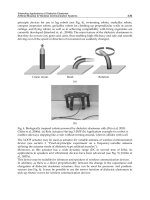
respectively. More signal-spectrum Fourier transform pairs can be found in the literature [1–3]. To
give some visual examples of real Fourier transforms, we have shown three most commonly referred
time waveforms and their Fourier transforms in Figure 2.9, where the square function, the triangular
function and the Gaussian function and their frequency-domain Fourier transforms are illustrated. As
they were generated from real spectrum plots from MATLAB, they are shown exactly as they should
appear in real applications.
Just as an oscilloscope is like a window in the time domain for observing signal waveforms, a
spectrum analyzer is a window in the frequency domain, generated by sweeping a filter across the
band of interest and detecting the power falling within the filter as it is swept. This power level can
then be plotted on the display of an oscilloscope. Usually, all spectra referred to in this book are
power spectra density (PSD) functions of the signals concerned. The relation between the PSD of a
signal and its Fourier transform can be written as
P(ω)=|F(ω)|
2
(2.21)
It is to be noted that the power of a signal can be calculated from either the time domain or the
frequency domain, and the results should be exactly the same as a consequence of power conservation

law.Thatis
1
2π

∞
−∞
P(ω)dω =

∞
−∞
|f(t)|
2
dt (2.22)
It is to be noted that the change of physical appearance in the time domain goes in the opposite
direction to that in the frequency domain. For instance, if we extend the duration of a signal waveform
FUNDAMENTALS OF WIRELESS COMMUNICATIONS 39
f(t)
f(t)
f(t)
1
1
1
F (w) = t
sin (wt/2)
wt/2
F (w) = t
F (w) = t
sin (wt/2)
wt/2
2p

t
2p
t
4p
t
4p
t
1
t
1
t
4p
t
t
2
t
2
4p
t
2p
t
t
t
−
2p
t
−
−
−
−

t
t
−
t
−
t
−
t
w
0
0
0
0
0
0
t
t
t
2
w
w
√
√
2pe
2p
(tw)
2
2
(a)
(b)

(c)
Figure 2.9 Fourier transform pairs for three commonly referred time waveforms. (a) Square wave-
form. (b) triangular waveform. (c) Gaussian waveform.
in the time domain, its Fourier transform will be compressed in the frequency domain, as stated
exactly in the scaling property of Fourier transform as follows:
f(at) ⇔
1
2π|a|
F

ω
2πa

(2.23)
where a is a scaling factor of time index variable t. The scaling factor a can be either more or less than
one, resulting in either compressed or extended original signal waveform of f(t)in the time domain.
The spectral bandwidth of a time-domain signal f(t) can be perfectly defined by the width in
frequency, at which its power is distributed. Therefore, the signal bandwidth is very much related to
the shape or appearance of its power spectra density function. Based on how much power is included
in its bandwidth, we have several different definitions of the signal bandwidth. The most commonly
used signal bandwidth is 3 dB signal bandwidth, which is defined as the width, over which the power
spectral density function falls from its peak value to a level 3 dB lower than the peak. This bandwidth
40 FUNDAMENTALS OF WIRELESS COMMUNICATIONS
is also called 3-dB bandwidth. The signal bandwidth can also be defined as the spectral width, over
which the included signal power becomes a fixed percentage of the total signal power. This can be
easily shown using the following expression as
99% ×
1
2π


∞
−∞
P(ω)dω =
1
2π

B
99%
−B
99%
P(ω)dω (2.24)
where B
99%
is the 99 percentage power bandwidth. Similarly, we can also define other percentage
power bandwidths,suchas90 percentage power bandwidth, 50 percentage power bandwidth,and
so on.
After having defined the signal bandwidth, we are ready to describe what an SS communication
system is in the sequel. Literally, an SS technique can be defined as any method for a transmitter to
spread the signal spectrum to a much wider extent than necessary to send the baseband signal itself
in a channel. At the receiver side, an SS receiver will be able to effectively collect most, if not all, of
the signal energy in a bandwidth spanned by the sent SS signal for effective detection. For instance,
a voice signal can be sent with amplitude modulation in a bandwidth roughly twice that of the voice
information itself. Other forms of modulation, such as low deviation FM or single sideband AM,
also permit information to be transmitted in a bandwidth comparable to the bandwidth of the sent
information itself. An SS system, however, often takes a baseband signal (e.g., a voice channel) with
a bandwidth of only a few kilohertz, and distributes it over a band that may span many megahertz
width in frequency. This is accomplished by modulating the information to be sent together with
a wideband encoding waveform, also called spread modulating signal. The most familiar example
of spectrum spreading is observed in conventional frequency modulation (FM), in which deviation
ratios greater than one are used. As a result, the bandwidth occupied by an FM modulated signal is

dependent on not only the information bandwidth but also the amount of modulation. As in all other
spectrum spreading systems, a signal-to-noise
6
advantage is gained by the modulation and demodu-
lation process. To measure the magnitude of this gained advantage, the terminology of process gain
is always used in an SS system.
Wideband FM could be considered as an SS technique from the standpoint that the carrier spec-
trum produced in the frequency modulation process is much wider than the transmitted information.
However, in the context of this section only those techniques are of interest in which some signal or
operation, other than the information being sent, is used for spreading the transmitted signal.
Many different spread spectrum techniques exist, in which the spreading codes or spreading
sequences will be used to control the frequency or time of transmission of the data-modulated carrier,
thus indirectly modulating the data-modulated carrier by the spreading codes or spreading sequences.
Several basic spread spectrum techniques available to the communications system designer will be
described and discussed in a general way in this part of Chapter 2. This section gives some detailed
descriptions of the various techniques and the signals generated. In addition to the most important (or at
least most prevalent) forms of SS modulation schemes (i.e., direct sequence (DS) spreading schemes),
other useful techniques such as frequency hopping (FH), time hopping, chirping and various hybrid
combinations of modulation forms will be described. Each is important in the sense that each has useful
applications. The historical tendency has been to confine each form to a particular application scenario.
Direct-sequence spreading, for instance, has been found most commonly used in civilian applications.
FH is more widely employed in military communication systems. Chirp modulation has been used
almost exclusively in radar. These systems will be discussed in the later subsections. The digital codes
or sequences used for the spreading signal will also be discussed in detail in Section 2.3 in this chapter.
There are four major techniques that will be accepted here as examples of SS signaling methods:
• Modulation of a carrier by a digital code sequence whose chip rate is much higher than the
information signal bandwidth. Such systems are called direct-sequence modulated systems.
6
Here, what we mean in “signal-to-noise” ratio is in fact “signal-to-interference” ratio, as no SS technique will
help to suppress noise, it will help suppress only interferences.

FUNDAMENTALS OF WIRELESS COMMUNICATIONS 41
• Carrier frequency shifting in discrete increments in a pattern determined by a code sequence.
This technique is called frequency hopping spread spectrum. The transmitter jumps from one
frequency to another in some predetermined sequence; the order of appearance of the frequen-
cies is determined by a controlling code sequence.
• The transmitted signal appears in different time slots within a fixed time frame, resulting in the
so called time hopping spread spectrum technique.
7
• Pulsed-FM or chirp modulation technique, in which a carrier is swept over a wide band during
a given pulse interval.
On the basis of the above four different SS techniques, many hybrid versions can be derived, such
as time-frequency hopping system, where the code sequence determines both the transmitted frequency
and the time of transmission, instead of only one as in the case of either FH or time hopping. Also, it
is to be noted that the pulse-FM or chirp modulation scheme was a direct derivation from the earlier
radar applications and not many applications have been found in modern communication networks
and systems due to its relatively low processing gain (PG) achievable and hard to use digital technique
for its signal processing.
Recently emerging UWB technologies have a lot in common with a time hopping SS system.
The UWB techniques will also use PPM to modulate digital signal (usually binary) with very nar-
row pulses. Therefore, the UWB technology is a further development of traditional SS systems.
More detail discussions on UWB technologies can be found in Section 7.6. Obviously, spread spec-
trum techniques form a foundation for modern CDMA technologies, which have been playing an
extremely important role in current 3G (and maybe beyond 3G as well) wireless networks and
communications.
In the following subsections, we will discuss the three major spread spectrum techniques, namely,
DS, FH, and time hopping techniques.
2.2.1 Direct-Sequence Spread Spectrum Techniques
The simplest method to spread the spectrum of a data-modulated signal is to modulate the signal a
second time using a wideband spreading signal, which always takes some forms of sequences, that is,
a pseudorandom sequence or PN sequence for short. This second modulation usually takes some form

of digital phase modulation, although analog amplitude or phase modulation is conceptually possible.
This spread spectrum (SS) scheme is called the direct sequence spread spectrum (DSSS) system, (or,
more exactly, directly carrier-modulated, code sequence modulation system) which is the best known
and most widely used spread spectrum system. This is because of their relative simplicity from the
point of view that they do not require a high-speed, fast-settling frequency synthesizer. Nowadays, DS
modulation has been used for commercial communication systems and measurement instruments, and
even laboratory test equipments that are capable of producing a choice of a number of code sequences
or operating modes. It is reasonable to expect that DS modulation will become a familiar form of
the spreading modulation scheme in many areas in the years to come due to its unique and desirable
features. Even now, commercial applications of DSSS systems are being explored. Characteristics of
DS spreading modulation is exactly the modulation of a carrier by a code sequence. In the general
case, the format may be AM, FM, or any other amplitude- or angle-modulation form. Very often,
however, the binary phase-shift keying (BPSK) is used, because it can be implemented at a very low
cost: only two balanced multiplication units are required, plus a low-pass filter followed by a decision
7
It has to be noted that one type of emerging ultra-wideband (also called UWB) technology works in a very
similar way as a time hopping SS. It is also called TH-UWB technology. Most commonly used modulation scheme
in the TH-UWB is pulse position modulation (PPM).
42 FUNDAMENTALS OF WIRELESS COMMUNICATIONS
device. The basic form of a DS signal is that produced by a simple and biphase-modulated (BPSK)
carrier. The details about the BPSK DSSS system will be introduced later.
The selection of spreading signals is of great importance in a DSSS system as it should have
certain properties that facilitate demodulation of the transmitted data signal by the intended receiver,
and make demodulation by an unintended receiver as hard as possible. These same properties will
also make it possible for the intended receiver to discriminate between the intended signal and jam-
ming, which usually appears quite differently from what is used for spreading the signal at the
transmitter. If the bandwidth of the spreading signal is much larger than the original data signal
bandwidth, the SS transmitting signal bandwidth will be dominated by the spreading signal and is
nearly independent of the original data signal. Each element of the spreading sequences or codes is
usually called a chip; its width will determine the bandwidth of the signal after spreading modula-

tion.
Before discussing any DSSS communication systems, we have to introduce the most important
characteristic parameter, namely, PG, which is defined as a function of the RF bandwidth of the DS
signal transmitted, compared with the bandwidth of its data information before carrier modulation.
The PG is exhibited as a signal-to-interference improvement resulting from the RF-to-information
bandwidth trade-off. It will also govern its capability to mitigate many other undesirable factors
appearing in the communication medium and signal detection processes, such as antijamming property,
and so on. The usual assumption is that the RF bandwidth is assumed to be equal to the main lobe of
the DS spectrum, which is always a
sin x
x
function. In many practical applications, the ratio between
the chip rate and original data information rate can also be used as the PG. Therefore, for a DSSS
system having a 10 Mcps chip rate and a 1 kbps information rate the PG will be (10
7
)/(10
3
) = 10
4
or about 40 dB. A more strict definition of the PG is given as
PG
DS
=
RF bandwidth of DS/SS signal
Baseband bandwidth of user data signal
(2.25)
∼
=
Chip rate of DS/SS signal
User data rate

The question arises then, whether the PG can be raised to a very high level to improve the
performance of a DSSS system. This question can be answered best by addressing the limitations
that exist with respect to expanding the bandwidth ratio to a arbitrarily large value so that the PG
may be increased indefinitely. Obviously, two parameters are available to adjust PG. The first is the
RF bandwidth, which depends on the chip rate used. For instance, if we have an RF (null-to-null)
bandwidth 100 MHz wide, the chip rate should be at least 50 Mcps. On this basis, how wide should
we make the system RF bandwidth and how much benefit can we obtain from the increase of the chip
rate? To double the RF bandwidth defined by the chip rate, we can only increase 3 dB PG. However,
the price is in its system complexity. With double the chip rate, the sampling rate at a digital receiver
has to be at least doubled. This will substantially increase the signal processing load at a DSP chip or
CPU. It is to be noted that the increase in the computation load is not linear with the increase in the
sampling rate. In other words, the doubling chip rate will probably result in trebling, quadrupling or
yielding an even higher computation load in a DSP chip. This imposes a great challenge to implement
real-time based communication applications, such as multimedia services. With the decrease in chip
duration (or increase in the chip rate) the smallest interval to make a decision at a receiver is also
reduced, leaving a result that the hardware and software have to catch up with the data rate to make a
sensible decision for each received bit on the basis of the chips. We should remember that the channel
characteristics never change with the increase of chip rate, as discussed in Section 2.1. With each
chip received at a receiver, all necessary algorithms, such as channel estimation, decision feedback,
equalization, and so on, have to be carried out and finished in time before the end of the chip in
question. It is still a great challenge to implement a full digital receiver at a chip rate 10 Gcps using
the state-of-the-art microelectronics technology. Thus, it is not a wise approach to increase the PG
FUNDAMENTALS OF WIRELESS COMMUNICATIONS 43
by using a higher chip rate. On the other hand, we can easily understand that it is not sensible to
increase the PG by reducing the user data rate either.
The most commonly used techniques for DS spreading are discussed below.
BPSK direct-sequence spread spectrum
The simplest form of DSSS employs BPSK as the spreading modulation. It has to be noted that here
we are talking about two modulations, that is, the spreading modulation and carrier modulation.The
former denotes the modulation of data information with a predetermined spreading code or sequence

to result in a bandwidth spreading, and the latter stands for modulating the baseband signal with a
high frequency radio carrier, only shifting the spectrum of the original baseband signal to a certain
RF frequency without yielding any bandwidth spreading. Therefore, for a BPSK DSSS system we
imply that the spreading modulation must be done using a BPSK modem. However, it is not certain
whether the carrier modulation in a BPSK DSSS system also employs the BPSK modem. As a matter
of fact, a BPSK DSSS system can also use any modem, such as BPSK, QPSK, MSK, and so on, for
its carrier modulation purpose.
Yet another important point we have to mention here is that the order of the spreading modulation
and carrier modulation is irreversible in most cases, and usually the spreading modulation happens
before the carrier modulation. In other words, the data signal should first be modulated by a spreading
signal, and then the spread signal will be further modulated by a radio frequency (RF) carrier before
being fed into the antenna for transmission. However, if both spreading modulation and carrier
modulation use BPSK modems, the order of the two become interchangeable.
Ideal BPSK modulation yields instantaneous phase shifts of the carrier by zero or 180 degrees
according to the signs of the binary data signal as a modulating signal. It can be mathematically
expressed by a multiplication of the carrier by a function c(i) that takes on the values ±1. Let us con-
sider a constant-envelope data-modulated carrier with power P , carrier radian frequency ω
c
,definedby
f
d
(t) =
√
2P cos
[
ω
c
t +φ
d
(t)

]
(2.26)
where φ
d
(t) stands for the data-modulated phase, which should take two different values, either zero
or 180 degrees depending on the signs (either +1or−1) of binary data information, and the term
√
2P is to give an average power P.
This signal occupies a bandwidth typically between one-half and twice the data rate prior to DS
spreading modulation, depending on the details of the data modulation and the pulse shapes used in
shaping the original data pulses. The BPSK spreading is accomplished by simply multiplying f
d
(t) by
a time-domain signal c(i) that is also called the spreading signal or spreading sequence, as illustrated
in Figure 2.10.
Binary
data signal
RF Carrier signal Spreading signal
c(t)
BPSK
carrier modulation
BPSK
spreading modulation
(2) (3)(2)
(1)
2P cos(w
c
t + f
d
)

√
2Pc(t)cos(w
c
t + f
d
)
√
2P cos w
c
t
√
Figure 2.10 Illustration of a BPSK DSSS transmitter.
44 FUNDAMENTALS OF WIRELESS COMMUNICATIONS
The transmitted signal after spreading modulation becomes
f
s
(t) =
√
2Pc(t)cos
[
ω
c
t +φ
d
(t)
]
(2.27)
whose bandwidth is basically determined by the spectral span of the spreading signal c(t),which
usually is a wideband spreading sequence. It is to be noted that the process of multiplication of c(t)
with f

d
(t) will not alter the power of the f
d
(t), but only extend the bandwidth of f
d
(t). This is what
an SS signal means. Then, we look back at the scaling property of the Fourier transform, which tells
us that the extension of the spectral span of a signal will equivalently make its time-domain waveform
shrink, just as expressed in Equation (2.23). From the power conservation law (Equation (2.22)), the
expansion in the bandwidth span of a signal in the frequency domain will reduce its peak amplitude
if the total power remains the same. This effect makes an SS signal appear like a wideband noise-
like interference to an unintended receiver. It is obvious that a conventional (non-spread-spectrum)
receiver would not be useful for detecting the wideband noise-like signal here because it is well
below the level of the real noise observed at the receiver.
The signal given in Equation (2.27) is transmitted into an AWGN channel with a transmission
delay τ
d
. The signal is received and contaminated by interference and channel AWGN noise. Demod-
ulation is accomplished in part by demodulating or remodulating with the spreading code locally
generated and appropriately delayed, c(t −˜τ
d
), as shown in Figure 2.11. This demodulation or corre-
lation of the received signal with the delayed spreading waveform is called the despreading process
and is an important function in any SS system. The signal after despreading the module in Figure 2.11
will become
r
1
(t) =
√
2Pc(t − τ

d
)c(t −˜τ
d
) cos
[
ω
c
t +φ
d
(t −τ
d
) + θ
]
(2.28)
where ˜τ
d
is the estimated delay at the receiver, τ
d
is the propagation delay that the transmitted signal
experienced, and θ is the phase delay caused by the propagation delay.
If the estimated delay at the receiver is exactly the same as the real delay, or ˜τ
d
= τ
d
,
Equation (2.28) will yield
√
2P cos
[
ω

c
t +φ
d
(t −τ
d
) + θ
]
(2.29)
as c(t −τ
d
)c(t −˜τ
d
) = 1if ˜τ
d
= τ
d
. This despread signal has been restored into a narrowband signal,
which is very similar to the original transmitted phase modulated data signal with only some difference
in the delay τ
d
and an extra phase θ caused by the propagation delay from the transmitter to the
receiver. This despreading process plays a crucial role here to transform the received wideband signal
into its original narrowband data signal.
Bandpass filter
Recoverd binary
data signal
Decision
device
Despreading signal
c(t − t

d
)
r
2
(t)r
1
(t)
Local carrier signal
+ noise + interference
2P cos(w
c
t)
√
√
~
2Pc(t − t
d
)cos[w
c
t + f
d
(t − t
d
) + q]
~~
(4)
(5)
(6)
Figure 2.11 Illustration of a BPSK DSSS receiver.
FUNDAMENTALS OF WIRELESS COMMUNICATIONS 45

On the other hand, if the receiver uses a wrong spreading signal or spreading sequence, say
c

(t −˜τ
d
), to despread the received wideband signal
√
2Pc(t −τ
d
) cos
[
ω
c
t +φ
d
(t −τ
d
) + θ
]
,it
will never accomplish the despreading process to restore the narrowband signal correctly, because
c(t − τ
d
)c

(t −˜τ
d
) will be another wideband sequence no matter whether ˜τ
d
= τ

d
or not and thus the
signal
√
2Pc(t − τ
d
)c

(t −˜τ
d
) cos
[
ω
c
t +φ
d
(t −τ
d
) + θ
]
(2.30)
will remain a wideband modulated signal. Therefore, the spreading signal c(t) is usually also called
the signature sequence or signature code as it behaves like a key to decode or despread the received
signal for recovering the original sent narrowband data signal.
There are six different time-domain waveforms observed at the transmitter and the receiver,
as shown in (1) to (6) in Figure 2.12. We can also allocate the corresponding observation points
from Figure 2.10 and Figure 2.11 accordingly, assuming that the binary data information in this case
(shown in Figure 2.12) is a constant value of +1 for illustration simplicity. We can then see how a
BPSK DSSS communication transceiver works step by step from the time-domain perspective.
The block diagrams shown in Figure 2.10 and Figure 2.11 illustrate a typical DSSS commu-

nications transceiver structure. It shows that a DSSS system can be viewed as a conventional
AM or FM communications link with only an extra part added to implement spreading modu-
lation and demodulation functionalities. In real applications the carrier modulation usually does
not happen before spreading modulation. The baseband information is digitized and added to the
spreading sequence first. For the discussion given in this section, however, we assume that the
RF carrier has already been data modulated before spreading modulation, because this can sim-
plify the discussion of the modulation-demodulation process in a BPSK DSSS system. After having
been amplified, a received signal is multiplied by a reference sequence generated at the receiver
locally and, given that the transmitter’s sequence and receiver’s sequence are synchronous and
the same, the carrier inversion phases (as shown in (3) and (4) in Figure 2.12) will be removed
successfully and the original carrier waveform will be restored. This narrowband restored car-
rier can then pass through a bandpass filter designed to pass only the original data-modulated
carrier.
(1) Carrier
Signals in DS transmitter Signals in DS receiver
(2) Spreading
sequence
(3) Spreading
modulated
carrier
(4) Received
DS modulated
signal
(5) Local
despreading
sequence
(6) Recovered
carrier
Figure 2.12 Conceptual illustration of time-domain signal waveforms for a BPSK DSSS transceiver.
The waveforms shown in this graph correspond to the observation points (1) to (3) in Figure 2.10

and the points (4) to (6) in Figure 2.11, respectively.
46 FUNDAMENTALS OF WIRELESS COMMUNICATIONS
All unwanted received signals are also treated by the same process at the receiver as the desired
signal, multiplying the received DS signal with a locally generated reference sequence. Any incoming
signal not synchronous with the receiver’s local reference sequence (a wideband signal) is spread to
a bandwidth still equal to the bandwidth of the received signal, because an unsynchronized input
signal is mapped into a bandwidth at least as wide as the receiver’s reference, such that the band-
pass filter can reject almost all the power of these undesired signals. This is the mechanism, by
which process gain is realized in a DSSS system; that is, the receiver transforms synchronous
input signals from the sequence-modulated bandwidth (wideband) to the data-modulated bandwidth
(narrowband). At the same time nonsynchronous input signals are spread at least over the spread-
ing sequence-modulated bandwidth. The data-modulated bandwidth specifies the bandwidth of a
bandpass filter followed by the decision device, and this bandpass filter in turn effectively con-
trols the amount of power from an unsynchronized or unwanted signal, which reaches the data
demodulator. We can see from the discussion here that the multiplication-and-filtering process before
data detection at the receiver provides the desired signal with an advantage or process gain.In
fact, the RF bandwidth in a DSSS system, as discussed earlier, directly affects many capabilities
of the system, such as how effectively it can reject external jamming. For instance, if a max-
imal 10-MHz bandwidth is available, the PG possible is also limited by that 10 MHz. Several
practical approaches are available in choosing the proper bandwidth in an anti-interception appli-
cation; the main interest is to minimize the power transmitted in terms of watts per Hertz. When
a maximum PG for interference rejection is needed, the bandwidth again should be made large
enough. If either frequency allocation or the propagation medium does not permit the use of a
wide RF bandwidth, some restraint must be applied. A prime consideration in SS systems (and
in particular, DS systems) is the bandwidth of the system with respect to the interference gener-
ated by other systems (that may not necessarily be SS systems) operating in the same or adjacent
channels.
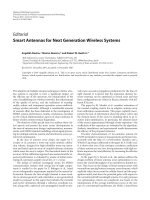
A conceptual spectral diagram of this type of DSSS signal format is shown in Figure 2.13, where
we only show the envelope of the PSD function of BPSK-modulated DSSS signal for illustration
clarity. The main lobe bandwidth (null-to-null) of the signal shown is usually equal to twice the

clock rate of the code sequence used as a spreading modulation signal. Each of the sidelobes has a
null-to-null bandwidth that is equal to the clock rate; that is, if the code sequence being used as a
modulating waveform has a 5 Mcps operating rate,
8
the main lobe of the null-to-null bandwidth will
be 10 MHz and each sidelobe will be 5 MHz wide. This is exactly the case in Figure 2.13. On the
other hand, in the time domain the BPSK-modulated DSSS carrier looks like the signal shown in
Figure 2.12, where the carrier is sent with zero phase shift when the code sequence is a +1, and a
180 degree phase shift when the code sequence is a −1.
To illustrate how a DSSS system works in the frequency domain, we would also like to look at
the issue from the perspective of power spectral density function as follows. Assume that the input
data information stream, as shown in Figure 2.10, is a random sequence with a transmission rate of
−20 −15 −50
PSD function
510 20
f (MHz)
15−10
Figure 2.13 Conceptual illustration of power spectral density function for BPSK DSSS signal. The
chip rate for this system is 5 Mcps and the null-to-null bandwidth of this DSSS system us 10 MHz.
8
Here, “Mcps” stands for mega chips per second.
FUNDAMENTALS OF WIRELESS COMMUNICATIONS 47
1
T
bit per second (bps), or
d(t) =
∞

k =−∞
d

k
p
T
(t −kT ) (2.31)
where d
k
=±1, the bit duration is T and p
T
(t) is the bit pulse waveform function. Thus, its power
spectral density (PSD) function ϕ
d
(f ) can be written into
ϕ
d
(f ) = T

sin fT
fT

2
(2.32)
whose shape is illustrated in Figure 2.14(a). Thus, it is seen from the figure that its bandwidth is just
equal to
1
T
Hz. Assume that the spreading sequence is also a random sequence and its chip rate is
1
T
c
. Therefore, its PSD function ϕ

c
(f ) can be expressed by
ϕ
c
(f ) = T
c

sin fT
c
fT
c

2
(2.33)
Assume T/T
c
= 4
A
2
T
c
/4
T
T
c
j
d
(f )
j
s

(f )
A
2
T/4
j
r
(f )
j
c
( f ) = j
cd
(f )
f
−1/T
c
1/T
c
2/T
c
2/T
−1/T 1/T0
−f
c
f
c
f
0
−f
c
f

c
f
0
(a) PSD functions for spreading sequence and data signal
(b) PSD function for BPSK spreading modulated signal
(c) The PSD for the carrier signal after despreading (r
1
(t) as shown in DS SS receiver)
Figure 2.14 The PSD functions for (a) original data and spreading sequence, (b) BPSK spreading
modulated signal, and (c) the carrier signal after despreading, where it is assumed that T = 4T
c
for
illustration clarity.
48 FUNDAMENTALS OF WIRELESS COMMUNICATIONS
which forms exactly the same expression as Equation (2.32) except for the interchange of bit duration
T and chip width T
c
. The PSD function for the spreading sequence ϕ
c
(f ) has also been drawn together
with the PSD function of data sequence ϕ
d
(f ) for easy comparison in Figure 2.14(a), where it is
assumed that T = 4T
c
for illustration clarity. Obviously, the bandwidth of spreading sequence is
equal to
1
T
c

Hz.
Now, let us consider the spreading modulation process as a simple multiplication between the
data signal and spreading sequence, resulting in a PSD function expressed by
ϕ
cd
(f ) = T
c

sin fT
c
fT
c

2
(2.34)
which takes exactly the same expression as Equation (2.33) and occupies the same bandwidth as
that of ϕ
c
(f ). In this way, the spreading modulation has extended the signal bandwidth to
T
T
c
= N
(N is assumed to be 4 in Figure 2.14) times. N is just equal to the PG of this DSSS system and is
usually a fairly large number. The carrier modulation after the spreading modulation will only shift
the spectrum ϕ
cd
(f ) to the center frequency f
c
, but never changes the physical appearance of ϕ

cd
(f ),
as shown in Figure 2.14(b).
The PSD function of transmitted signals from the antenna of the transmitter becomes
ϕ
s
(f ) =
PT
c
2


sin(f −f
c
)T
c
(f − f
c
)T
c

2
+

sin(f +f
c
)T
c
(f +f
c

)T
c

2

(2.35)
which is a bandpass signal and its bandwidth is
2
T
c
Hz, as shown in Figure 2.14(b). It is observed
from the figure that the amplitude of ϕ
s
(f ) is reduced by
2T
PT
c
if compared with ϕ
d
(f ); whereas the
width of ϕ
s
(f ) increases N =
T
T
c
(which is just the PG value) times if compared with ϕ
d
(f ).
At the DSSS receiver, the PSD function of the received signal has the same PSD function of

the transmitted signal, with only a delay and some extra phase also caused by propagation delay,
as shown in Figure 2.11. The delay will never change the shape of the PSD function. It is easy to
show that the PSD function of the signal after the despreading process, or signal r
1
(t) as indicated
in Figure 2.11, can be written as
ϕ
r
(f ) =
PT
2


sin(f −f
c
)T
(f − f
c
)T

2
+

sin(f +f
c
)T
(f +f
c
)T


2

(2.36)
which has been plotted in Figure 2.14(c). It is to be noted that the Equation (2.36) has exactly the
same expression as ϕ
s
(f ), as written in Equation (2.35), except for the interchange of T
c
and T .
It is not surprising to us as the despreading process at the receiver will restore the original data
signal bandwidth, such that most of its power can pass easily through the bandpass filter, as shown
in Figure 2.11. It is seen from the figure that, similar to the ϕ
d
(f ), the PSD function ϕ
r
(f ) spans
also a narrowband spectrum with its bandwidth being
2
T
, which is just the double of that for signal
d(t). The spectrum ϕ
r
(f ) will be restored into a narrowband baseband PSD function after the carrier
demodulation, which just shifts its center frequency from f
c
back to zero.
QPSK direct-sequence spread spectrum
It is a well-known fact that the use of quadrature modulation scheme can effectively improve the
bandwidth efficiency of a digital modem without sacrificing the power efficiency. The two quadrature
carriers, that is, sin(ω

c
t) and cos(ω
c
t), are perfectly orthogonal due to the simple fact that

∞
−∞
sin(ω
c
t)cos(ω
c
t)dt =

2π
0
sin(ω
c
t)cos(ω
c
t)dt = 0 (2.37)
FUNDAMENTALS OF WIRELESS COMMUNICATIONS 49
It is interesting that we cannot find more carriers than these two, that is, sin(ω
c
t) and cos(ω
c
t),
which possess such an ideal orthogonality. For instance, in a orthogonal frequency division multiplex-
ing (OFDM) system we can use many subcarriers to send data information in parallel. However, those
subcarriers are not orthogonal in a strict sense as each subcarrier is always overlapped by half with its
two neighboring subcarriers and this half-overlapping in the same signal space will introduce serious

interferences in many circumstances, such as in the case of being under the influence of the multipath
effect and Doppler effect. However, the two quadrature carriers, sin(ω
c
t) and cos(ω
c
t), can work in
a much more robust way against many channel impairments without affecting their perfect orthogo-
nality due to the property that their orthogonality is not established in the same signal space. Instead,
their orthogonality is based in a two-dimensional space, that is, in-phase and quadrature spaces, which
are vertical with each other,
9
as shown in Figure 2.15. Therefore, it is seen that the carriers sin(ω
c
t)
and cos(ω
c
t) can always keep their orthogonality even under many undesirable operational conditions
because they move in different signal spaces, which are already perfectly orthogonal to each other.
The use of QPSK modulation in a digital modem can double the bandwidth efficiency with its power
efficiency kept unchanged.
The same idea can be applied to a DSSS system to improve its bandwidth efficiency when com-
pared with a BPSK DSSS system. However, it has to be noted that the use of in-phase and quadrature
channels in a QPSK DSSS system should consider the issues on spreading codes or sequences assign-
ment problem, that is, should we assign two different codes to In-phase and quadrature channels, or
use the same code for the two channels? Therefore, a QPSK DSSS system should not be considered
equivalently as a normal QPSK digital modulation system.
To illustrate the issue clearly, let us consider a generic QPSK DSSS transmitter and a receiver, as
shown in Figure 2.16 and Figure 2.17, respectively. d(t) is the input information data stream defined
in Equation (2.31) with its duration being T , c
1

(t) and c
2
(t) are two spreading sequences generated
in the transmitter for I and Q channel spreading modulations, A sin(2πf
c
t +θ) and A cos(2πf
c
t +θ)
are in-phase and quadrature carriers for QPSK modulation, where the average power of the carrier is
P =
A
2
2
and θ is the initial phase of the carriers.
In-phase
signal space
Radian frequency
cos w
c
t
sin w
c
t
Quadrature
signal space
w
c
w
Figure 2.15 Orthogonality of sin(ω
c

t) and cos(ω
c
t) carriers in the in-phase and quadrature signal
spaces in QPSK digital modulation.
9
We say the two signal spaces are vertical to each other to imply that they have π/2 phase difference.
50 FUNDAMENTALS OF WIRELESS COMMUNICATIONS
d(t)c
1
(t)
d(t)c
2
(t)
s(t) = s
1
(t) + s
2
(t)
c
1
(t)
s
1
(t)
s
2
(t)
d(t)
c
2

(t)
BPSK
QPSK DS SS signal
+
BPSK
Acos(2 pf
c
t + q)
Asin(2 pf
c
t + q)
90° shift
Sequence generator 1
Sequence generator 2
2A sin(2pf +q+g (t))
√
=
Figure 2.16 A generic QPSK DSSS transmitter.
s(t−t)
c
1
(t − t)
c
2
(t − t)
u
1
(t)
u
2

(t)w
2
(t)
w
1
(t)
Z
i
u(t)
Recovered
data
(.) dt
t + l
i
+ T
t + l
i
A sin(2 pf
c
t + q′)
A cos(2 pf
c
t + q′)
+
−
∫
Figure 2.17 A generic QPSK DSSS receiver.
From Figure 2.16, the QPSK DSSS signal can be expressed as
s(t) = s
1

(t) + s
2
(t)
= Ad(t )c
1
(t) sin(2πf
c
t +θ) + Ad(t)c
2
(t) cos(2πf
c
t +θ)
=
√
2A sin(2πf
c
t +θ + γ(t)) (2.38)
where the phase modulated component can be written into
γ(t) = arctan
c
2
(t)d(t)
c
1
(t)d(t)
=






















π
4
, if c
1
(t)d(t) =+1andc
2
(t)d(t) =+1
3π
4
, if c
1
(t)d(t) =−1andc
2

(t)d(t) =+1
5π
4
, if c
1
(t)d(t) =−1andc
2
(t)d(t) =−1
7π
4
, if c
1
(t)d(t) =+1andc
2
(t)d(t) =−1
(2.39)
FUNDAMENTALS OF WIRELESS COMMUNICATIONS 51
1
1
0
−1
0
−1
−1
d(t)
c
1
(t)
2TT
1

c
2
(t)
0
−1
1
0
−1
1
0
0
0
0
−1
−A
−A
−
A
A
2A
d(t)c
1
(t)
d(t)c
2
(t)
s
1
(t)
s

2
(t)
s(t)
t
t
t
t
t
t
t
t
√
2A
√
g = 7p/4
3p/4 3p/4 3p/47p/4 7p/4p/45p/4 5p/4p/4
Figure 2.18 Signal waveforms in a generic QPSK DSSS transceiver.
It is seen from Equation (2.39) that s(t) will yield four different phases: θ +
π
4
, θ +
3π
4
, θ +
5π
4
and θ +
7π
4
, according to different combinations of d(t)c

1
(t) and d(t)c
2
(t). Figure 2.18 illustrates
the signal waveforms in different points of a QPSK DSSS transceiver. It is noted that two different
spreading sequences c
1
(t) and c
2
(t) have been used here to plot Figure 2.18. Of course, there are
other alternatives for the assignments of the two spreading sequences in both I and Q channels,
resulting in a very different overall performance, implementation complexity, and other characteristic
features of the QPSK DSSS system in question. For instance, we can also choose to use the same
spreading sequence for spreading modulations in both I and Q channels. In doing so, we will have the
advantage that less sequences will be needed for each user in order to support more users in the same
spread spectrum multiple access (SSMA) network.
10
The use of the same spreading sequence in both
I and Q channel spreading modulations is also allowed since the in-phase and quadrature channels
employ two orthogonal carriers, sin(2πf
c
t +θ) and cos(2πf
c
t +θ), which have already ensured a
good isolation between the two channels. However, extra protection will be given if in-phase and
quadrature channels use two different spreading sequences, in case some cross-talk between the I
10
It is to be noted that the two acronyms, SSMA and CDMA, are interchangeable in some cases. The former
emphasizes the wideband nature of SS techniques; whereas the later the user division mechanism by codes.
52 FUNDAMENTALS OF WIRELESS COMMUNICATIONS

and Q channels exists due to nonideal operational effects, such as the frequency or phase estimation
inaccuracy or jitter in the local oscillator of a QPSK DSSS receiver. The price paid to have this extra
protection is that the number of spreading sequences needed for the whole SSMA network will be
doubled, and in many cases the family size of an appropriate spreading sequences suitable for such a
multiple access application is always limited. This issue will be addressed in detail in Section 2.3.3.
The receiver for this generic QPSK DSSS system is shown in Figure 2.17, where it is assumed that
the receiver knows the exact propagation delay from the transmitter and receiver or τ and will generate
two different spreading sequences c
1
(t −τ)and c
2
(t −τ)accordingly. In this case, the receiver should
carry out despreading before carrier demodulation, corresponding to the order of spreading modulation
and carrier modulation carried out in the transmitter. As a QPSK modem can be viewed as two BPSK
modems working in parallel, we can understand that the order of spreading modulation and carrier
modulation can be interchanged in both transmitter and receiver at the same time. It means in this
case that we can also first perform carrier modulation before spreading modulation at the transmitter,
and thus first have carrier demodulation before the despreading operation at the receiver.
We also assume that the receiver knows the initial phases θ

of the in-phase and quadrature carriers
in the received signal s(t − τ) such that it can regenerate the local carrier references A sin(2πf
c
t +θ

)
and A cos(2πf
c
t +θ


) that are in-phase with the received signal, resulting in a coherent QPSK DSSS
signal reception. It is to be noted that the difference between the initial phases θ of the in-phase
and quadrature carriers at the transmitter and the initial phases θ

at the receiver is due to the signal
propagation delay through the channel.
After the despreading and carrier demodulation process, the signals from the I and Q channels
will be combined and undergo integration in a unit, which functions like a low-pass filter to remove
higher frequency harmonics generated in the carrier demodulation process. The integration will take
place within the duration of the ith data bit of interest from τ + t
i
to τ + t
i
+ T ,wheret
i
is the
starting time of the ith bit and τ is the propagation delay. The output from the integrator will form
a decision variable Z
i
.
In the following illustration of basic operation of a DSSS receiver we will only concern ourselves
with a simple LOS propagation path and will not take into account other channel impairing factors,
such as multipath effect, Doppler effect, and so on, for illustration simplicity. Therefore, the received
signal can be written as
s(t − τ) = Ad(t − τ)c
1
(t −τ)sin

2πf
c

t +θ


+ Ad(t − τ)c
2
(t −τ)cos

2πf
c
t +θ


(2.40)
where the initial phase can be also expressed by θ

= θ − 2πf
c
τ and τ is the propagation delay in
the transmission path from the transmitter to the receiver. The signals in the I and Q channels after
despreading and carrier demodulation become
u
1
(t) = Ad(t − τ)sin
2

2πf
c
t +θ



+ Ad(t − τ)c
1
(t −τ)c
2
(t −τ)sin

2πf
c
t +θ


cos

2πf
c
t +θ


=
A
2
d(t − τ)

1 −cos(4πf
c
t +2θ

)

+

A
2
d(t − τ)c
1
(t −τ)c
2
(t −τ)sin(4πf
c
t +2θ

) (2.41)
and
u
2
(t) = Ad(t − τ)cos
2

2πf
c
t +θ


+ Ad(t − τ)c
1
(t −τ)c
2
(t −τ)sin

2πf
c

t +θ


cos

2πf
c
t +θ


FUNDAMENTALS OF WIRELESS COMMUNICATIONS 53
=
A
2
d(t − τ)

1 +cos(4πf
c
t +2θ

)

+
A
2
d(t − τ)c
1
(t −τ)c
2
(t −τ)sin(4πf

c
t +2θ

) (2.42)
respectively. The summation of the signals from the I and Q channels will become
u(t) = u
1
(t) + u
2
(t)
= Ad(t − τ) + Ad(t − τ)c
1
(t −τ)c
2
(t −τ)sin(4πf
c
t +2θ

) (2.43)
Obviously, after the low-pass filtering, the second term in Equation (2.43) will vanish and only
the term Ad(t − τ) reflecting the data information remains, yielding the decision variable Z
i
= AT
if +1issentorZ
i
=−AT if −1 is sent. Therefore, the strength of the decision variable generated
from a QPSK DSSS receiver is just equal to the twice that generated from a single BPSK DSSS
receiver if they work under the same condition (i.e., most importantly, their data transmission rates
should be kept the same), implying a 3 dB increase in the signal-to-noise-ratio (SNR). It is to
be noted that this gain in the SNR does not pay any price in bandwidth efficiency as both the

I and Q channels occupy the same bandwidth, which is exactly the same as the bandwidth for a
BPSK DSSS system. This is really wonderful and can happen only using the two unique orthogonal
carriers sin(2πf
c
t) and cos(2πf
c
t). It is a pity that we cannot find any more such ideal orthogonal
carriers.
The two spreading sequences c
1
(t) and c
2
(t) applied to the I and Q channels can be two different
ones or split up from one same sequence c(t), as shown in Figure 2.19, where the chip duration of
c(t) is half of that for either c
1
(t) or c
2
(t), and thus the length of either c
1
(t) or c
2
(t) is only the half
of that of c(t).
Basically, the bit error rate (BER) performance of a QPSK DSSS system is the same as that of
a BPSK DSSS system. In fact, either the I or the Q channel can be viewed effectively as a single
BPSK DSSS system and each of them possesses the same BER as a normal BPSK DSSS system.
Therefore, two BPSK systems (in the QPSK DSSS system in question) working together will yield
the same BER as a single BPSK system.
c(t)

c
1
(t)
t
t
t
c
2
(t)
1
1
−1
1
−1
−1
Figure 2.19 Split up of one sequence into two spreading sequences for their use in a QPSK DSSS
system.
54 FUNDAMENTALS OF WIRELESS COMMUNICATIONS
However, the bandwidth efficiency of a QPSK DSSS system is double that of a single BPSK
DSSS system, and it can be explained as follows. Assume that T
c
is the chip width for both c
1
(t) and
c
2
(t). Thus, s
1
(t) and s
2

(t) will have the same bandwidth equal to
2
T
c
. This QPSK DSSS system has
its data transmission rate of
1
T
and the PG of PG =
T
T
c
. The bandwidth of this QPSK DSSS system
is determined by the chip width of c
1
(t) and c
2
(t).
It is to be noted that the I and Q channels in the transmitter shown in Figure 2.16 send the same
information bit stream with its data rate of
1
T
. However, we can also use the I and Q channels to
deliver different data information to increase the transmission rate to
2
T
, if the bit duration in the I
and Q channels is kept unchanged. In this case, the receiver structure should be modified to detect
the data information in the I and Q channels separately. The modified block diagrams for a QPSK
DSSS system with double data rate are shown in Figure 2.20 and Figure 2.21, respectively.

There are the following factors that will affect the performance of a QPSK DSSS system: trans-
mission rate or bandwidth, PG and SNR (or transmission power). In order to compare the performance
of two DSSS systems, such as a BPSK system and a QPSK DSSS system, we have to concentrate
on one particular parameter, with the other two fixed, to make the comparison easily and objectively.
For instance, if we want to compare BPSK and QPSK DSSS systems shown in Figures 2.10 and
2.20, we should fix the data rate and PG first (thus the bandwidth), allowing us to make a fair com-
parison on SNR values for the two schemes. Since the same data rate is concerned, the bit duration
in either the I or Q channel in Figure 2.20 will be twice as wide as that in Figure 2.10. Also due to
S/P
BPSK
BPSK
90° shift
Sequence generator 1
Sequence generator 2
d(t)
c
1
(t)
d
1
(t)c
1
(t)
d
2
(t)c
2
(t)
c
2

(t)
s
1
(t)
s
2
(t)
A sin(2 pf
c
t + q)
A cos(2 pf
c
t + q)
s(t) = s
1
(t) + s
2
(t)
QPSK DSSS signal
2A sin(2pf + q+g(t))
√
=
Figure 2.20 An alternative structure of QPSK DSSS transmitter with double transmission rate.
s(t−t)
c
1
(t − t)
c
2
(t − t)

u
1
(t)
u
2
(t)w
2
(t)
w
1
(t)
Z
i
Z
i
Recovered
data
P/S
A sin(2 pf
c
t + q′)
A cos(2 pf
c
t + q′)
+
−
+
−
(.) dt
t + l

i
+ T
t + l
i
∫
(.) dt
t + l
i
+ T
t + l
i
∫
Figure 2.21 An alternative structure of QPSK DSSS receiver with double transmission rate.
FUNDAMENTALS OF WIRELESS COMMUNICATIONS 55
the fact that the same PG value is assumed for the two schemes, we can readily conclude that the
bandwidth efficiency (defined by bit/s/Hz) for the two schemes should be the same. However, the
power efficiency of the QPSK DSSS system shown in Figure 2.20 is double that of a BPSK DSSS
system shown in Figure 2.10, due to its wider bit duration and high signal power available for the
detection of each bit in the QPSK scheme, implying a higher SNR value.
The DSSS systems using other modulation schemes, such as MSK, QAM and so on, can also
be studied using a similar methodology as illustrated in this subsection. Those who are interested in
them can refer to these references [255–268].
As a final remark before the end of this subsection, it is to be noted that one of the most
successful applications for the QPSK DSSS techniques is the GPS system [244–254], which was
launched initially in the United States for positioning applications in military operations. Nowadays,
the GPS has found a worldwide applications in various practical systems, most of which are civilian
applications and services.
2.2.2 Frequency Hopping Spread Spectrum Techniques
Another method to spread the spectrum of a data-modulated carrier is to switch the carrier frequency
from one to another periodically. Usually, each carrier frequency is selected from a set of frequencies,

which are spaced approximately as the same width of the data modulation bandwidth. The spreading
code in this case does not directly modulate the data-modulated carrier but is instead used to control
the appearance sequence of carrier frequencies. Because the transmitted signal appears as a data-
modulated carrier which is hopping from one frequency to another, this type of spread spectrum is
called frequency hopping spread spectrum (FHSS). In the receiver, the FH is removed by mixing
(down-converting) with a local oscillator signal that is hopping synchronously with the received
signal.
Based on its function and behavior, the FHSS technique is more accurately termed as, code-
controlled multifrequency-FSK modulation. It works very similar to a conventional frequency shift
keying (FSK) modulation scheme, except that the set of frequencies is very large. On the other hand,
a normal FSK modem often uses only two frequencies. For instance, f
1
is sent to denote a mark,
f
2
is to signify a space. In the FH schemes, there will be thousands of frequencies available. The
number at a few hundreds to thousands is normal in a real system, which makes discrete frequency
selections randomly on the basis of a predetermined sequence in combination with the data information
conveyed. The number of frequencies and the rate of hopping from frequency to frequency in an
FHSS system is determined by operational requirements for a particular communication application.
The basic structure of an FHSS system can be described as follows. Usually, a FH system must
have a sequence generator and a frequency synthesizer, which is capable of generating the corre-
sponding frequencies according to the sequence generator. It is difficult to develop an FHSS system
to design a fast-settling frequency synthesizer with a sufficient large number of carrier frequencies.
Theoretically speaking, the instantaneous frequency output, the frequency synthesizers generate, must
be a single frequency.
11
However, a practical system may produce an output spectrum, which can be
a composite of the desired frequency, sidebands generated by hopping, as well as some other spurious
frequencies generated as by-products.

Figure 2.22 shows a conceptual block diagram of a FHSS transmitter. The receiver of an FHSS
system is given in Figure 2.23. The waveforms generated by this simple FHSS system (in both
transmitter and receiver) are shown in Figure 2.24, where it is assumed that the data information is
kept at the same level (here all bits are +1 constantly) for simplicity of illustration.
11
This is one of the reasons that make a FH system costly and very difficult to implement. In particular, the
frequency synthesizer in a fast hopping FH system has to work to switch from one frequency to another in a very
fast and stable way, especially when the data rate is very high.
56 FUNDAMENTALS OF WIRELESS COMMUNICATIONS
User data
d(t)
Data
modulation
Bandpass
filter
Acosw
c
t
Frequency
synthesizer
Sequence
generator
(b)
(a)
Figure 2.22 Conceptual block diagram of a FHSS transmitter.
Front
filter
Bandpass
filter
Data

demodulator
Recovered data
Frequency
synthesizer
Sequence
generator
Acosw
I
t
(c)
(e)
(d)
d(t)
∼
Figure 2.23 Conceptual block diagram of a FHSS receiver.
The FHSS transmitter shown in Figure 2.22 consists of the following basic blocks: a data mod-
ulator, a mixer (denoted simply by a multiplier in the figure), a FH patter sequence generator, a
frequency synthesizer, a bandpass filter and an antenna. The data modulator will perform the dig-
ital modulation between the user data d(t) and a carrier A cos ω
c
t,whereA is its amplitude. The
frequency synthesizer will work according to the hopping sequences generated by the sequence gener-
ator. Usually, the sequence generator can produce a great number of different patterns, each of which
will be used by the frequency synthesizer to generate a particular carrier, which will be multiplied
with the data-modulated signal in the mixer to produce an up-converted transmitting signal from
the antenna. Therefore, the carrier frequency of the transmission signal is under the control of the
sequence generator, which can also control the FH rate from one frequency to another. The hopping
rate is a very important parameter in a FHSS system, which will determine if it is a fast hopping or
slow hopping FH system.
At the FHSS receiver, as shown in Figure 2.23, the received signal should first go through a

front-end filter, which will be used to reject the image of the carrier frequency produced in the
mixer. For the same purpose, the sequence generator will produce a replica of the sequence used
by the transmitter and will yield a FH pattern, which should be exactly the same as that used in
the transmitter, in the output of the frequency synthesizer. The locally generated FH pattern will be
FUNDAMENTALS OF WIRELESS COMMUNICATIONS 57
(a)
(b)
(c)
(d)
(e)
w
I
w
1
+ w
I
w
2
+ w
I
w
3
+ w
I
w
4
+ w
I
w
1

w
2
w
3
w
4
Figure 2.24 Waveforms generated in different points of the FHSS transmitter (as shown in
Figure 2.22) and the receiver (as shown in Figure 2.23). (a) The output sequence generated in hop-
ping pattern sequence generator; (b) the output signal from the frequency synthesizer; (c) sequence
generated in the local sequence generator at the receiver; (d) the local carrier waveforms generated
by the local frequency synthesizer; (e) The carrier output from the mixer of the receiver.
mixed with the received signal to produce a narrowband data-modulated signal with a fixed carrier
frequency, which should be equal to the intermediate frequency (IF) ω
I
. The output IF signal will be
demodulated by a data demodulator to recover the transmitted data information or
˜
d(t).
Ideally, the spectrum generated from a FH system should be perfectly rectangular, with spectral
lines distributed evenly in every predetermined frequency channel. The transmitter should also be
designed to send the same amount of power in each frequency. Otherwise, the detection efficiency
on different frequencies will be uneven, causing decision errors at the receiver.
As shown in Figure 2.23, the received frequency hopping signal is mixed with a locally generated
replica, which is offset by a fixed amount (which is equal to a carrier frequency) suitable for reception
process at the receiver, ω
I
) such that the output from the mixer in the receiver will produce a constant
difference frequency ω
I
if the transmitter and receiver code sequences are synchronous.

58 FUNDAMENTALS OF WIRELESS COMMUNICATIONS
As in the case of the DSSS system discussed in Section 2.2.1, any signal that is not a replica
of the local reference is spread by multiplication with the local reference, not being restored into
its original narrowband waveform. Bandwidth of an undesired signal after multiplication with the
local reference is approximately equal to the bandwidth before despreading. For instance, an external
sinusoidal signal received at a FH receiver will be converted into a signal that will change in the
same way as the local reference (a FH carrier), and thus it will never pass the bandpass filter, which
is tuned to a fixed carrier frequency or IF, say ω
I
. On the other hand, if a desirable signal appears at
the input side of the receiver, the output signal from the FH despreading unit will be a narrowband
signal modulated by a fixed carrier ω
I
, which will undergo a data demodulation process to recover
the original data information sent or
˜
d(t), as shown in Figure 2.23.
Processing gain of a FH system
The IF mixer and the bandpass filter in the transmitter are effective to reject undesired signal power
that lies outside its bandwidth defined by the useful data signal bandwidth. Because this IF bandwidth
is only a fraction of the bandwidth of the local FH carrier reference, it can be seen that almost all
the undesired signal’s power is rejected, whereas a desirable signal is enhanced by being correlated
with the local FH carrier reference. In Section 2.2.1, it was illustrated that a DSSS system operates
identically from the viewpoint of undesired signal rejection and restoration of the desired signal. From
this general point of view, DS and FH systems are similar. However, they are different in the details
of their operation. Like the PG defined in the DSSS system, we should also define the PG for the
FHSS system, and this value will also play an extremely important role in determining the overall
performance of a FH system.
The PG of the FH systems should be defined for two different cases. One case is that all gen-
erated carrier frequencies are contiguous, and the other is noncontiguous. The noncontiguous carrier

frequencies are common for applications when it is hard to find enough spectrum allocation for the
FHSS communications. On the other hand, the contiguous carrier frequencies are the ideal situations,
which can simplify the calculation of the PG. By the contiguous FH spectrum, we mean that all the
carrier frequencies generated by the synthesizer are evenly spaced in the frequency domain.
The PG of a FH system with a contiguous spectrum can be calculated in the same way as a DSSS
system. That is,
PG
FH
=
BW
RF
BW
information
(2.44)
where BW
RF
is the bandwidth spanned by all the carrier frequencies generated by the synthesizer
collectively, and BW
nformation
is the bandwidth given by the original baseband information signal,
which is determined by the data signal d(t).
On the other hand, if the carrier frequencies generated by the synthesizer are not contiguous, an
objective measure of PG can be
PG
FH
= the total number of available frequencies (2.45)
which can also be used to calculate the PG value for a FH system with contiguous carrier channels. For
example, a FH system containing 1000 frequencies can have 30 dB available PG. The approximation
has been used in the simple calculation for PG, given in Equation (2.44), because all guard bands in
between two carrier channels are neglected in the formula. If the guard bands in the IF bandwidth

cannot be omitted, Equation (2.45) should be used instead.
Hopping rate of a FH system
The FH rate and number of carrier frequencies are determined by the sequence generator. The mini-
mum frequency switching rate of a FHSS system is determined by the following system parameters:
FUNDAMENTALS OF WIRELESS COMMUNICATIONS 59
• The bandwidth of information to be sent and its importance.
• The amount of redundancy needed.
• The environment where the FH system will work in terms of severity of the interferences.
Information in a FH system can be sent in any way available to the other systems. Usually,
however, some form of digital signal is preferred, whether the information is a digitized analog
signal or data. Assume for the present that some digital rate is prescribed and that FH has been
chosen as the SS technique. Then, the question is how to determine the FH rate or the chip rate. It is
to be noted that, in contrast to a DS system, there is no chip in a FH system. The term chip is used
here just for conceptual analogy.
A FH system should possess a sufficiently large number of frequencies on demand. The number
required depends on the operational environment of the system. For example, two thousand frequen-
cies will provide satisfactory operation when interference and noise are evenly distributed at every
available frequency channel. For equal distribution of interference or jammers in every channel, the
interference power required to block communications has to approach two thousand times that of the
desired signal power. In other words, the achievable jamming margin is about 33 dB in this case.
Unless some sort of redundancy that allows for bit decisions based on more than one frequency is
needed, a single narrowband interferer will cause an error rate of 0.5 × 10
−3
, which is generally
satisfactory for normal digital data transmission. For a simple FH system without any form of trans-
mitted data redundancy (one hop exists in each bit duration), the expected error probability can be
approximated by
J
N
,whereJ is equal to the number of CW interferers whose power is greater than

or equal to signal power, and N is the number of frequencies available to the FH system. Error rate
probability for a FH system, in which we assume that binary FSK modulation is used (here two
frequencies denote binary symbols or f
1
=+1andf
0
=−1), can be approximated by the following
expansion
P
e
=
N
c

n=r

N
c
r

p
n
q
N
c
−n
(2.46)
where p is the error probability of a single jamming trial, which is J/N, J denotes the number of
jamming carriers, N is the number of channels available to the FH system, q is the probability of
no error for a single jamming trial (we always have q = 1 −p), N

c
is the number of hops in each
bit,
12
r is the number of wrong chip decisions necessary to cause a bit error. A chip decision error is
defined as the situation where interference power in a “+1” channel exceeds the power in an intended
“−1” channel (or vice versa) by some amount ε that is sufficient to cause a decision error.
A FH system is called a slow frequency hopping spread spectrum system if only one or less than
one hop happens in each bit /symbol duration. Otherwise, if more than one hopping exists, a fast
frequency hopping system results.
A fast hopping FH system can offer a much better performance than that of a slow hopping FH
system at the price of system implementation complexity. For instance, the implementation cost for
a fast hopping FH system with three hops per bit will be at least three times more complex than that
of a slow hopping FH system with one hop per bit. The synthesizer should work at least three times
faster than that of a one-hop-per-bit system. The amount of data a transceiver should process should
also be at least three times more than that of an one-hop-per-bit system.
The performance of a three-hop-per-bit FH system can be evaluated by the following method.
Assume that the decision rule for this system is on the basis of the two out of three decision rule.
12
The value of N
c
will determine fast FH or slow FH. Often, N
c
can be a noninteger. For instance, N
c
= 1/2
means that one hopping happens in every two bits, implying a slow FH system. On the other hand, if N
c
> 1, a
fast FH system is the resultant.

60 FUNDAMENTALS OF WIRELESS COMMUNICATIONS
That is if at least two frequencies are correct, the decision will be made in favor of the symbol or
bit representing the FH patterns containing the two correct frequencies. Thus, a single jamming trial
will cause not more than

3
2

p
2
q
3−2
= 3p
2
q (2.47)
where

n
m

denotes the number of combinations of taking m from n items, p and q represent the
probability of error caused by a single jamming trial and the probability of no error caused by a
single jamming trial, respectively, and p = 1 − q. Consider a FH system with totally two thousands
carrier frequencies, p will be
1
2000
and q = 1 − p = 0.9995. Thus, the error probability will become
3

1

3000

2

1 −
1
3000

∼
=
7.5 ×10
−7
, which is much better than 0.5 × 10
−3
given by the previous one
hop -per bit FH system.
Due to the limited space, we will not discuss the FHSS Systems further. For more information
on FHSS, please refer to the references [269–307].
2.2.3 Time Hopping Spread Spectrum
and Ultra-Wideband Techniques
After having discussed the two popular SS techniques, DS and FH, we would also like to give a brief
introduction of the third SS technique, time hopping (TH) technique, in this subsection.
The TH technique, in fact, works in a very similar way as a digital modulation scheme called pulse
position modulation (PPM). In other words, time hopping is nothing but a type of pulse position modu-
lation in a sense that a code sequence is used to key the transmitter on and off, as shown in Figure 2.25,
where the times for the transmitter to switch on and off follow a specific pseudorandom code sequence.
The average duty cycle of “on” and “off ” in the transmitter can become as large as 0.5. The major
difference between the PPM and the TH lies in the fact that the former uses pulse position patterns
to represent the data information symbols, whereas the latter denotes a particular code sequence,
which acts as a secret key to further decode the data information hidden therein. A conceptual block

diagram of a TH system is shown in Figure 2.25, where the on–off switch logic unit in the transmitter
is used to control the positions that the sent pulse will hop from one to the other. The receiver in
Figure 2.25(b) should also follow exactly the same hopping pattern to capture all transmitted power
from the transmitter. Obviously, an unintended receiver will not be able to receive all power from a
User data
On–off switch
logic
Pulse
modulator
On-pulse
gate
Off-pulse
gate
On-pulse
detector
On-pulse
detector
Recovered
user data
Sequence
generator
Sequence
generator
(a) Time hopping spread spectrum transmitter (b) Time hopping spread spectrum receiver
Decision
device
Figure 2.25 Block diagram of a THSS transceiver, where the sequence generator is used to control
the TH patterns that should change synchronously in both the transmitter and the receiver.