Báo cáo y học: "Differential expression analysis for sequence count data" ppt

MET H O D Open Access
Differential expression analysis for sequence
count data
Simon Anders
*
, Wolfgang Huber
Abstract
High-throughput sequencing assays such as RNA-Seq, ChIP-Seq or barcode counting provide quantitative readouts
in the form of count data. To infer differential signal in such data correctly and with good statistical power,
estimation of data variability throughout the dynam ic range and a suitable error model are required. We propose a
method based on the negative binomial distribution, with variance and mean linked by local regression and
present an implementation, DESeq, as an R/Bioconductor package.
Background
High-throughpu t seque ncing of DNA fragment s is used
in a range of quantitative assays. A common feature
between these assays is that they sequence large
amounts of DNA fragments that reflect, for example, a
biological system’s repertoire of RNA molecules (RNA-
Seq [1,2]) or the DNA or RNA interaction regions of
nucleo tide binding molecules (ChIP-Seq [3], HITS-CLIP
[4]). Typically, these reads are assigned to a class based
on their mapping to a common region of the target gen-
ome, where each class represents a target transcript, in
the case of RNA-Seq, or a binding region, in the case of
ChIP-Seq. An important summary statistic is the num-
ber of reads in a class; for RNA-Seq, this read count has
been found to be (to good approximation) linearly
related to the abundance of the target transcript [2].
Inter est lies in comparing read counts between different
biological conditions. In the simplest case, the compari-
son is done separately, class by class. We will use the

term gene synonymously to class, even though a class
may also refer to, for example, a transcription factor
binding site, or even a barcode [5].
We would like to use statistical testing to decide
whether, for a given gene, an observed difference in
read counts is significant, that is, whether it is greater
than what would be expected just due to natural
random variation.
If reads were independently sampled from a popula-
tion with given, fixed fraction s of genes, the read counts
would follow a multinomial distribution, which can be
approximated by the Poisson distribution.
Consequently, the Poisson distribution has been used
to test for differential expression [6,7]. The Poisson dis-
tribution has a single parame ter, which is uniquely deter-
mined by its mean; its variance and all other properties
follow from it; in particular, the variance is equal to the
mean. Howev er, it has been noted [1,8] that the assump-
tion of Poisson distribution is too restrictive: it predicts
smaller variations than what is seen in the data. There-
fore, the resulting statistical test does not control type-I
error (the probability of false discoveries) as advertised.
We show instances for this later, in the Discussion.
To address this so-called overdispersion problem, it has
been proposed to model count data wit h negative bino-
mial (NB) distributions [9], and this approach is used in
the edgeR package for analysis of SAGE and RNA-Seq
[8,10]. The NB distribution has parameters, which are
uniquely determined by mean μ and variance s
2

.How-
ever, the number of replicates in data sets of interest is
often too small to estimate both p arameters, mean and
variance, reliably for each gene. For edgeR,Robinson
and Smyth assumed [11] that mean and variance are
related by s
2
= μ + aμ
2
, with a single proportionality
constant a that is the same throughout the experiment
and that can be estimated from the data. Hence, only
one parameter needs to be estimated for each gene,
allowing application to experiments with small numbers
of replicates.
In this paper, we extend this model by allowing more
general, data-driven relationships of variance and mean,
provide an effective algorithm for fitting the model to
* Correspondence:
European Molecular Biology Laboratory, Mayerhofstraße 1, 69117 Heidelberg,
Germany
Anders and Huber Genome Biology 2010, 11:R106
/>© 2010 Anders et al This is an open access article distributed under the terms of the Cre ative Commons Attribution L icense (http://
creativecommons.or g/licenses/by/2.0), which permits unrestricted use, distribution, and reproduction in any medium, provided the
original work is properly cited.
data, and show that it provides better fits (Section
Model). As a result, more balanced selection of differen-
tially expressed genes throughout the dynamic range of
the data can be obtained (Section Testing for diffe rential
expression). We demonstrate the method by applying

it to four data sets (Section Applications)anddiscuss
how it compare s to alternative approaches (Section
Conclusions).
Results and Discussion
Model
Description
We assume that the number of reads in sample j that
are assigned to gene i can be modeled by a negative
binomial (NB) distribution,
K
ij ij ij
~(,),NB

2
(1)
which has two parameters, the mean μ
ij
and the
variance

ij
2
. The read counts K
ij
are non-negative
integers. The probabilities of the distribution are given
in Supplementary Note A. (All Supplementary Notes are
in Additional file 1.) The NB distribution is co mmonly
used to model count data when overdispersion is
present [12].

In practice, we do not know the parameters μ
ij
and

ij
2
, and we need to estimate them from the data.
Typically, the number of replicates is small, and further
modelling assumpti ons need to be made in order to
obtain useful esti mates. In this paper, we develop a
method that is based on the following three assumptions.
First, the mean parameter μ
ij
, that is, the expectation
value of the observed counts for gene i in sample j,is
the product of a condition-dependent per-gene value q
i,
r(j)
(where r(j) is the experimental condition of sample
j) and a size factor s
j
,


ij
ijj
q
S
=
,()

.
(2)
q
i,r(j)
is proportional to the expectation value of the
true (but unknown) concentration of fragments from
gene i under condition r(j). The size factor s
j
repre sents
the coverage, or sampling depth, of library j, and we will
use the term common scale for quantities, such as q
i, r(j)
,
that are adjusted for coverage by dividing by s
j
.
Second, the variance

ij
2
is the sum of a shot noise
term and a raw variance term,


ij ij j i j
sv
22
=+
shot noise
raw variance



,()
.
(3)
Third, we assume that the per-gene raw variance
parameter v
i, r
is a smooth function of q
i
, r,
vvq
ij ij,() ,()
().

=
(4)
This assumption is needed because the number of
replicates is typically too low to get a precise estimate of
thevarianceforgenei fromjustthedataavailablefor
this gene. This assumption allows us to pool the data
from genes with similar expression strength for the pur-
pose of variance estimation.
The decomposition of the variance in Equation (3) is
motivated by the following hierarchical model: We
ass ume that the actua l concentration of fragments from
gene i in sample j is proportional to a random variable
R
ij

, such that the rate that fragments from gene i are
sequenced is s
j
r
ij
. For each gen e i and all samples j of
condition r,theR
ij
are i.i.d. with mean q
ir
and variance
v
ir
. Thus, the count value K
ij
, conditioned on R
ij
= r
ij
,is
Poisson distributed with rate s
j
r
ij
. The marginal distribu-
tion of K
ij
- when allowing for variation in R
ij
-hasthe

mean μ
ij
and (according to the law of total variance) the
variancegiveninEquation(3).Furthermore,ifthe
higher moments of R
ij
are modeled according to a
gamma distribution, the marginal distribution of K
ij
is
NB (see, for example, [12], Section 4.2.2).
Fitting
We now describe how the model can be fitted to data. The
data are an n × m table of counts, k
ij
,wherei = 1 , , n
indexes the genes, and j =1, ,m indexes the samples. The
model has three sets of parameters:
(i) m size factors s
j
; the expectation values of all
counts from sample j are proportional to s
j
.
(ii) for each experimental condition r, n expression
strength parameters q
ir
; they reflect the expected abun-
dance of fragments from gene i under condition r,that
is, expectation values of counts for gene i are propor-

tional to q
ir
.
(iii) The smooth functions v
r
:R
+
® R
+
; for each con-
dition r, v
r
models the dependence of the raw variance
v
ir
on the expected mean q
ir
.
Thepurposeofthesizefactorss
j
is to render
counts from different samples, w hich may have been
sequenced to different depths, com parable. Hence, the
ratios (

K
ij
)/(

K

ij’
) of expected counts for the same
gene i in different samples j and j’ should be e qual to
thesizeratios
j
/s
j’
if gene i is not differentially
expressed or samples j and j’ are replicates. The total
number of reads, Σ
i
k
ij
, may seem to be a good measure
of sequencing depth and hence a reasonable choice for
s
j
. Experience with real data, however, shows this not
always to be the case, because a few highly and differ-
entially expressed genes may have strong influence on
the total read count, causing the ratio of total read
countsnottobeagoodestimatefortheratioof
expected counts.
Anders and Huber Genome Biology 2010, 11:R106
/>Page 2 of 12
Hence, to estimate the size factors, we take the median of
the ratios of observed counts. Generalizing the procedure
just outlined to the case of more than two samples, we use:
s
k

k
j
i
ij
iv
v
m
m
^
/
.=
⎛
⎝
⎜
⎞
⎠
⎟
=
∏
median
1
1
(5)
The denominator of this expression can be interpreted
asapseudo-referencesampleobtainedbytakingthe
geometric mean across samples. Thus, each size factor
estimate
s
j
^

is computed as the median of the ratios of
the j-th sample’s counts to those of the pseudo-reference.
(Note: While this manuscript was under review, Robinson
and Oshlack [13] suggested a similar method.)
To estimate q
ir
, we use the average of the counts from
the samples j corresponding to condition r, transformed
to the common scale:
q
m
k
s
i
ij
j
jj
^
^
:()
,



=
=
∑
1
(6)
where m

r
is the number of replicates of condition r and
the sum runs over these replicates. the functions v
r
,we
first calculate sample variances on the common scale
w
m
k
s
q
i
ij
j
i
jj




=
−
−
⎛
⎝
⎜
⎜
⎜
⎞
⎠

⎟
⎟
⎟
=
∑
1
1
2
^
^
:()
(7)
and define
z
q
m
s
i
i
j
jj




=
=
∑
^
^

:()
.
1
(8)
In Supplementary Note B in Additional file 1 we show
that w
ir
- z
ir
is an unbiased estimator for the raw variance
parameter v
ir
of Equation (3).
However, for small numbers o f replicates, m
r
,asis
typically the case in applications, the values w
ir
are highly
variable, and w
ir
- z
ir
would not be a useful variance
estimator for statistical inf erence. Instead, we use local
regression [14] on the graph
(, )
^
qw
i

i


to obtain a
smooth function w
r
(q), with
vq wq z
ii
i
^^ ^
() ()





=−
(9)
as our estimate for the raw variance.
Some attention is needed to avoid estimation biases in
the local regression. w
ir
is a sum of squared random
variables, and the residuals
wwq
i
i



− ()
^
are skewed.
Following References [15], Chapter 8 and [14], Section
9.1.2, we use a generalized linear model of the gamma
family for the local regression, using the implementation
in the locfit package [16].
Testing for differential expression
Supposethatwehavem
A
replicate samples for biologi-
cal condition A and m
B
samples for condition B. For
each gene i, we would like to weigh the evidence in the
data for differential expression of that gene between
the two conditions. In particular, we would like to test
the null hypothesis q
iA
= q
iB
, where q
iA
is the expression
strength parameter for the samples of condition A, and
q
iB
for condition B. To this end, we define, as test statis-
tic, the total counts in each condition,
KKKK

iij
jj
iij
jj
A
A
B
B
==
==
∑∑
:() :()
,,

(10)
and their overall sum K
iS
= K
iA
+ K
iB
. From the error
model described in the previous Section, we show below
that - under the null hypothesis - we can compute the
probabilities of the events K
iA
= a and K
iB
= b for any
pair of numbers a and b.Wedenotethisprobabilityby

p (a, b). The P value of a pair of observed count sums
(k
iA
, k
iB
) is then the sum of all probabilities less or equal
to p(k
iA
, k
iB
), given that the overall sum is k
iS
:
p
pab
pab
i
abk
pab pk k
abk
i
ii
i
=
+=
≤
+=
∑
∑
(,)

(,)
.
(,) ( ),
S
AB
S
(11)
The variables a and b in the above sums take the
values 0, , k
iS
. The approach presented s o far follows
that of Robinson and Smyth [11] and is analogous to
that taken by other conditioned tests, such as Fisher’s
exact test. (See Reference [17], Chapter 3 for a discus-
sion of the merits of conditioning in tests.)
Computation of p(a, b). First, assume that, under the
null hypothesis, counts from different samples are inde-
pendent. Then, p(a, b)=Pr(K
iA
= a)Pr(K
iB
= b). The
problem thus is computing the probability of the event
K
iA
= a, and, analogously, of K
iB
= b. The random vari-
able K
iA

is the sum of m
A
NB-distributed random variables. We approximate i ts
distribution by a NB distribution whose parameters we
obtain from those of the K
ij
.Tothisend,wefirstcom-
pute the pool ed mean estimate from the counts of both
conditions,
qks
i
ij
jj AB
j
^
:(){ ,}
/,
0
=
∈
∑

(12)
Anders and Huber Genome Biology 2010, 11:R106
/>Page 3 of 12
which accounts for the fact that the null hypothesis
stipulates that q
iA
= q
iB

. The summed mean and var-
iance for condition A are

^
^
,
i
j
j
i
sq
A
A
=
∈
∑
0
(13)

^
^^
^
^^
().
i
j
j
i
j
i

sq
s
vq
A
A
A
2
0
2
0
=+
∈
∑
(14)
Supplementary Note C in Additional file 1 describes
how the distribution parameters of the N B for K
iA
can
be determined from

^
iA
and

^
iA
2
.(Toavoidbias,we
do not match the moments directly, but instead match a
different pair of distribution statistics.) The parameters

of K
iB
are obtained analogously.
Supplementary Note D in Additional file 1 explains
how we evaluate the sums in Equation (11).
Applications
Data sets
We present results based on the following data sets:
RNA-Seq in fly embryos. B. Wilczynski, Y H. Liu,
N. Delhomme and E. F urlong have conducted RNA-Seq
experiments in fly embryos and kindly shared part of their
data with us ahead of publication. In each samp le of this
data set, a gene was engineered to be over-expressed, and
we compare two biologic al replicates each of two such
conditions, in the following denoted as ‘A’ and ‘B’.
Tag-Seq of neural stem cells. Engström et al. [18] per-
formed Tag-Seq [19] for tissue cultures of neural cells,
including four from glioblastoma-derived neural stem-
cells (’GNS’) and two from non-cancerous neural stem
( ’ NS’ ) cells. As each tissue culture was derived from a
different subject and so has a different genotype, these
data show high variability.
RNA-Seq of yeast. Nagalakshmi et al. [1] performed
RNA -Seq on replicates of Saccharomyces cerevisiae cul-
tures. They tested two library preparation protocols , dT
and RH, and obtained three sequencing runs for each
protocol, such that for the first run of each protocol,
they had one furthe r technical replicate (same culture,
replicated library preparation) and one further biological
replicate (different culture).

ChIP-Seq of HapMap samples. Kasowski et al. [20]
compared protein occupation of DNA regions between
ten human individuals by ChIP-Seq. They compiled
a list of regions for polymerase II and NF-B, and
counted, for each sa mple, the number of reads that
mapped onto each region. The aim of the study was to
investigate how much the regions’ occupation differed
between individuals.
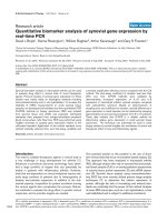
Variance estimation
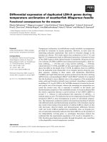
We start by demonstrating the variance estimation.
Figure 1a shows the sample variances w
ir
(Equation (7))
plotted against the means
q
i
^

(Equation (6)) for condi-
tion A in the fly RNA-S eq data. Also shown is the local
regression fit w
r
(q) and the shot noise
sq
j
i
^^

. In Figure
1b, we plotted the squared coefficient of variation

(SCV), that is the ratio of the variance to the mean
squared. In this plot, the distance between the orange
and the purple line is the SCV of the noise due to biolo-
gical sampling (cf. Equation (3)).
ThemanydatapointsinFigure1bthatliefarabove
the fitted orange curve may let the fit of the local
regression appear poor. However, a strong skew of the
residual distribution is to be expected. See Supplemen-
tary Note E in Additional file 1 for details and a discus-
sion of diagnostics suitable to verify the fit.
Testing
In order to verify that DESeq maintains control of type-I
error, we contrasted one of the replicates for condition
A in the fly data against the other one, using for both
samples the variance function estimated from the two
replicates. Figure 2 shows the empirical cumulative dis-
tribution functions (ECDFs) of the P values obtained
from this comparison. To c ontrol type-I error, the pro-
portion of P values below a threshold a has to be ≤ a,
that is, the ECDF curve (blue line) should not get above
the diagonal (gray line). As the figure indicates, type-I
error is controlled by edgeR and DESeq,butnotbya
Poisson-based c
2
test. The latter underestimates the
variability of the data and would thus make many false
positive rejections. In addit ion to this evaluation on real
data, we also verified DESeq’s type-I error control on
simulated data that were generated from the error
model described above; see S upplementary Note G in

Additional file 1. Next, we contrasted the two A samples
against the two B samples. Using the procedure
described in the previous Section, we computed a
P value for each gene. Figure 3 shows the obtained fold
changes and P values. 12% of the P values were below
5%. Adjustment for multiple-testing with the procedure
of Benjamini and Hochberg [21] yielded significant dif-
ferential expression at false discovery rate (FDR) of 10%
for 864 genes (of 17,605). These are marked in red in
the figure. Figure 3 demonstrates how the ability to
detect differential expression depends on overall coun ts.
Specifically, the strong shot noise for low counts causes
the testing procedure to call only very high fold changes
significant. It can also be seen that, for counts below
approximat ely 100, even a small increase in count levels
reduces the impact of shot noise and hence the fold-
change requirement, while at higher counts, when
shot noise becomes unimportant (cf. Figure 1b), the
Anders and Huber Genome Biology 2010, 11:R106
/>Page 4 of 12
Figure 1 Dependence of the variance on the mean for condition A in the fly RNA-Seq data. (a) The scatter plot shows the common-scale
sample variances (Equation (7)) plotted against the common-scale means (Equation (6)). The orange line is the fit w(q). The purple lines show the
variance implied by the Poisson distribution for each of the two samples, that is,
sq
j
iA
^^
,
. The dashed orange line is the variance estimate used by
edgeR. (b) Same data as in (a), with the y-axis rescaled to show the squared coefficient of variation (SCV), that is all quantities are divided by the

square of the mean. In (b), the solid orange line incorporated the bias correction described in Supplementary Note C in Additional file 1. (The plot
only shows SCV values in the range [0, 0.2]. For a zoom-out to the full range, see Supplementary Figure S9 in Additional file 1.)
p value
Empirical CDF
0.0
0.5
1.0
DESeq, below 100
0.0 0.5 1.0
DESeq, above 100
DESeq, all
edgeR, below 100
edgeR, above 100
0.0
0.5
1.0
edgeR, all
0.0
0.5
1.0
0.0 0.5 1.0
Poisson, below 100
Poisson, above 100
0.0 0.5 1.0
Poisson, all
p value
Empirical CDF
0.00
0.02
0.04

0.06
0.08
DESeq, below 100
0.00 0.04 0.08
DESeq, above 100
DESeq, all
edgeR, below 100
edgeR, above 100
0.00
0.02
0.04
0.06
0.08
edgeR, all
0.00
0.02
0.04
0.06
0.08
0.00 0.04 0.08
Poisson, below 100
Poisson, above 100
0.00 0.04 0.08
Poisson, all
 


Figure 2 Type-I error control. The panel s show empir ical cumulative distribution functions (ECDFs) f or P values from a comparison of one
replicate from condition A of the fly RNA-Seq data with the other one. No genes are truly differentially expressed, and the ECDF curves (blue)
should remain below the diagonal (gray). Panel (a): top row corresponds to DESeq, middle row to edgeR and bottom row to a Poisson-based c

2
test. The right column shows the distributions for all genes, the left and middle columns show them separately for genes below and above a
mean of 100. Panel (b) shows the same data, but zooms into the range of small P values. The plots indicate that edgeR and DESeq control type I
error at (and in fact slightly below) the nominal rate, while the Poisson-based c
2
test fails to do so. edgeR has an excess of small P values for low
counts: the blue line lies above the diagonal. This excess is, however, compensated by the method being more conservative for high counts. All
methods show a point mass at p = 1, this is due to the discreteness of the data, whose effect is particularly evident at low counts.
Anders and Huber Genome Biology 2010, 11:R106
/>Page 5 of 12
fold-change cut-off depends only weakly on count level.
These plots are helpful to guide experiment design: For
weakly expressed gene s, in the region where shot noise
is important, power can be increased by deeper sequen-
cing, while for the higher-count regime, increased power
can only be achieved with further biological replicates.
Comparison with edgeR
We also analyzed the data with edgeR (version 1.6. 0;
[8,10,11]). We ran edgeR with four different settings,
namely in common-dispersion and in tagwise-dispersion
mode, and either using the size factors as estimated by
DESeq or taking the total numbers of sequenced reads.
The results did not depend much on these c hoices, and
here we report the results for tag-wise dispersion mode
with DESeq-estimated size factors. (The R code required
to reproduce a ll analyses, figures and numbers reported
in this ar ticle is provided in Add itional file 2; in addi-
tion,thissupplementprovidestheresultsforthe
other settings of edgeR. The raw data can be found in
Additional file 3.)

Going back to Figure 1 we see that edgeR’ ssingle-
value dispersion estimate of the variance is lower than
that of DESeq for weakly expressed genes and higher for
strongly expressed genes. As a cons equence, as we have
seen in Figure 2edgeR is anti-conservative f or lowly
expressed genes. However, itcompensatesforthisby
being more conservative with strongly expressed genes,
so that, on average, type-I error control is maintained.
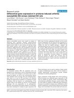
Nevertheless, in a test between different conditions,
this behavior can result in a bias in the list of discov-
eries; for the present data, as Figure 4 shows, weakly
expressed genes seem to be overrepresented, while very
few genes with high average level are called differentially
expressed by edgeR. While overall the sensitivity of both
methods seemed comparable (DESeq reported 864 hits,
edgeR 1, 127 hits), DESeq produced results which were
more balanced over the dynamic range.
Similar results were obtained with the neural stem cell
data, a data set wit h a different biological background
and different noise c haracteristics (see Supplementary
Note F in Additional file 1). The flexibility of the var-
iance estimation scheme present ed in this work appears
to offer real advantages over the existing methods across
a range of applications.
Working without replicates
DESeq allows analysis of experiments with no biological
replicates in one or even b oth of the conditions. While
one may not want to draw strong conclusions from
such an analysis, it may still be useful for exploration
and hypothesis generation.

If replicates are available only for one of the conditions,
one might choose to assume that the variance-mean
dependence estimated from the data for that condition
holds as well for the unreplicated one.
If neither condition has replicates, one can still per-
form an analysis based on the assumption that for most
genes, there is no true differential expression, and th at a
valid mean-variance relationship can be estimated from
treating the two samples as if they were replicates. A
minority of differen tially abundant genes will act as out-
liers; however, they will not have a severe impact on the
gamma-family GLM fit, as the gamma distribution for
low values of the shape parameter has a heavy right-
hand tail. Some overestimation of the variance may be
expected, which will make that approach conservative.
We performed such an analysis with the fly RNA-Seq
and the neural cell Tag-Seq data, by restricting both
data sets to only two samples, one from each condition.
For the neural cell data, the estimated variance function
was, as expected, somewhat above the two function s
estimated from the GNS and NS replicates.
Using it to test for differential expression still found
269 hits at FDR = 10%, of which 202 were among the
612 hits from the more reliable analysis with all avail-
able samples. In the case of the fly RNA-Seq data, how-
ever, only 90 of the 862 hits (11%) were recovered (with
two new hits). These observations are explained by
the fact that in the neural cell d ata, the variability
between replicates was not muc h smaller than between
Figure 3 Testing for differential expression between conditions

A and B: Scatter plot of log
2
ratio (fold change) versus mean.
The red colour marks genes detected as differentially expressed at
10% false discovery rate when Benjamini-Hochberg multiple testing
adjustment is used. The symbols at the upper and lower plot
border indicate genes with very large or infinite log fold change.
The corresponding volcano plot is shown in Supplementary Figure
S8 in Additional file 2.
Anders and Huber Genome Biology 2010, 11:R106
/>Page 6 of 12
conditions, making the latter a usable surrogate for the
former. On the other hand, for the fly data, the variabil-
ity between replicates was much smaller than between
the conditions, indicating that the replication provided
important and otherwise not available information on
theexperimentalvariationinthedata(seealsonext
Section).
Variance-stabilizing transformation
Given a variance-mean dependence, a variance-stabiliz-
ing transformation (VST) is a monotonous mapping
such that for the transformed values, the variance is
(approximately) independent of the mean. Using the
variance -mea n dependenc e w(q) estimated by DESeq,a
VST is given by


()
()
.=

∫
dq
wq
(15)
Applying the transformation τ to the common-scale
count data, k
ij
/s
j
, yields values whose variances are
approximately the same throughout the dynamic range.
One application of VST is sample clustering, as in
Figure 5; such an approach is more straightforward
than, say, defining a suitable distance metric on the
untransforme d count data, whose choice is not obvious,
and may not be easy to combine with available cluster-
ing or classificat ion algorithms (which tend to be
designed for variables with similar distributional
properties).
ChIP-Seq
DESeq can also be used to analyze comparative ChIP-
Seq assays. Kasowski et al. [20] analyzed transcription
factor binding for HapMap individuals and counted for
each sample how many reads mapped to pre-determined
binding regions. We considered two individuals from
their data set, HapMap IDs GM12878 and GM12891,
for both of which at least four replicates had been done,
and tested for differential occupation of the regions. The
upper left two panels of Figure 6 which show compari-
sons within the same individual, indicat e that type-I

error was controlled by DESeq. No region was signifi-
cant at 10% FDR using Benjamini-Hochberg adjustment.
Differential occupation was found, h owever, when con-
trasting the two individuals, with 4,460 of 19,028 regions
significant when only two replicates each were used and
8,442 when four replicates were used (uppe r right two
panels).
Using an alternative approach, Kasowski et al. fitted
generalize d linear models (GLMs) of the Poisson family.
This (lower row of Figure 6) resulted in an enrichment
of small P values even for comparisons within the same
individual, indicating that the variance was underesti-
mated by the Poisson GLM, and literal use of the P
values would lead to anti-conservative (overly optimistic)
bias. Kasowski et al. addressed this and adjusted for the
bias by using additional criteria for calling differential
occupation.
Conclusions
Why is it necessary to develop new statistical metho-
dology for sequence count data? If large numbers of
replicates were available, questions of data distribution
could be avoided by using non -parametric methods,
such as rank-based or permutation tests. However, it
is desirable (and possible) to consider experiments
with smaller numbers of replicates per condition.
In order to compare an obse rved difference with an
expected random variation, we can improve our pic-
ture of the latter in two ways: first, we can use distri-
bution families, such as normal, Poisso n and negative
binomial distributions, in order to determine the

higher moments, and hence the tail behavior, of statis-
tics for differential expression, based on observed low
order moments such as me an and variance. Second,
we can share information, for instance, distributional
parameters, between genes, based on the notion that
data from different genes f ollow similar patterns of
variability. Here, we have described an instance of
such an approach, and we will now discuss the choices
we have made.
Choice of distribution
While for large counts, normal distributions might
provide a good approximation of between-replicate
variability, this is not the case for lower count values,
whose discreteness and skewness mean that probability
estimates c omputed from a normal approximation
would be inadequate.
For the Poisson approximation, a key paper is the
work by Marioni et al. [6], who studied the technical
−10123456
0.00 0.02 0.04
lo
g
10 mean
d
ens
i
ty
x7
Figure 4 Distribu tion of hits th rough the dynamic range.The
density of common-scale mean values q

i
for all genes in the fly
data (gray line, scaled down by a factor of seven), and for the hits
reported by DESeq (red line) and by edgeR at a false discovery rate
of 10% (dark blue line: with tag-wise dispersion estimation; light
blue line: common dispersion mode).
Anders and Huber Genome Biology 2010, 11:R106
/>Page 7 of 12
reproducibility of RNA-Seq. They extracted total RNA
from two tissue samples, one from the liver and one
from the kidneys of the same individual. From each
RNA sample they took seven aliquots, prepared a library
from each aliquot according to the protocol recom-
mended by Illumina and sampled each library on one
lane of a Solexa genome analyzer. For each gene, they
then calculated the variance of the seven counts from
the same tissue sample and found very good agreement
with the variance predicted by a Poisson model. In line
with our arguments in Section Model, Poisson shot noise
is the minimum amount of variation to expect in a
counting process. Thus, Marioni et al. concluded that the
technical reproducibility of RNA-Seq is excellent, and
that the variation between technical replicates is close to
the shot noise limit. From this vantage point, Marioni
et al. (and s imilar ly Bullard et al. [22]) suggested to use
the Poisson model (and Fisher’s exact test, or a likelihood
ratio test a s an approximat ion to it) to test whether a
gene is differentially expressed between their two s am-
ples.Itisimportanttonotethatarejectionfromsucha
test only informs us that the difference between the aver-

age counts in the two samples is larger than one would
expect between technical replicates. Hence, we do not
G
liNS1
G144
CB660
CB541
G166
G179
GNS (L
)
GNS
NS
NS
GNS (*)
GNS (*)
0 100 200
Value
Color Key
Figure 5 Sample clustering for the neural cell data of Kasowski et al. [18]. A common variance function was estimated for all samples and
used to apply a variance-stabilizing transformation. The heat map shows a false colour representation of the Euclidean distance matrix (from
dark blue for zero distance to orange for large distance), and the dendrogram represents a hierarchical clustering. Two GNS samples were
derived from the same patient (marked with ‘(*)’) and show the highest degree of similarity. The two other GNS samples (including one with
atypically large cells, marked ‘(L)’) are as dissimilar from the former as the two NS samples.
Anders and Huber Genome Biology 2010, 11:R106
/>Page 8 of 12
know whether this difference is due to the different tissue
type, kidney instead of liver, or wheth er a difference of
the same magnitude could have been found as well if one
had compared two sa mples from different parts of the

same liver, or from livers of two individuals.
Figure 1 shows that shot noise is only dominant for
very low count values, while already for moderate
counts, the effect of the biological variation between
samples exceeds the shot noise by orders of magnitude.
This is confirmed by comparison of technical with bio-
logical replicates [1]. In Figure 7 we used DESeq to obtain
variance estimates for the data of Nagalakshmi et al. [1].
The analysis indicates that the difference between techni-
cal replicates barely exceeds shot noise level, while biolo-
gical replicates differ much more. Tests for diffe rential
expression that are based on a Poisson model, such as
those discussed in References [6,7,20,22,23] should thus
be interpreted with caution, as they may severely under-
estimate the effect of biological variability, in particular
for highly expressed genes.
Consequently, i t is preferable to use a model
that allows for overdispersion. While for the Poisson
distribution, variance and mean are equal, the negative
binomial distribution is a generalization that a llow for
the variance to be larger. The most advanced of the
published methods using this distribution is likely edgeR
[8]. DESeq owes its basic idea to edgeR,yetdiffersin
several aspects.
Sharing of information between genes
First, we discovered that the use of total read counts as
estimates of sequencing depth, and hence for the adjust-
ment of observed counts between samples (as recom-
mended by Robinson et al. [8] and others) may result in
p value

Empirical CDF
0.0
0.5
1.0
D: A1 vs A2
0.0 0.5 1.0
D: B1 vs B2 D: A1 vs B1
0.0 0.5 1.0
D: A vs B
0.0 0.5 1.0
P: A1 vs A2 P: B1 vs B2
0.0 0.5 1.0
P: A1 vs B1
0.0
0.
5
1.0
P: A vs B
Figure 6 ApplicationtoChIP-Seqdata.ShownareECDFcurvesforP values resulting from comparisons of Pol-II ChIP-Seq data between
replicates of the same individual (first and second column) and between two different individuals (third and forth column). The upper row
corresponds to an analysis with DESeq (’D’), the lower row to one based on Poisson GLMs (’P’). If no true differential occupation exists (that is,
when comparing replicates), the ECDF (blue) should stay below the diagonal (gray), which corresponds to uniform P values. In the first column,
two replicates from HapMap individual GM12878 (A1) were compared against two further replicates from the same individual (A2). Similarly, in
the second column, two replicates from individual GM12891 (B1) were compared against two further replicates from the same individual (B2).
For DESeq, no excess of low P values was seen, as expected when comparing replicates. In contrast, the Poisson GLM analysis produced strong
enrichments of small P values; this is a reflection of overdispersion in the data, that is, the variance in the data was larger than what the Poisson
GLM assumes (see also Section Choice of distribution). The third column compares two replicates from individual GM12878 (A1) against two from
the other individual (B1). True occupation differences are expected, and both methods result in enrichment of small P values. The forth column
shows the comparison of four replicates of GM12878 (A1 combined with A2) against four replicates of GM12891 (B1, B2); increased sample size
leads to higher detection power and hence smaller P values.

Anders and Huber Genome Biology 2010, 11:R106
/>Page 9 of 12
hig h app arent differences between replicates, and hence
in poor power to detect true differences.
DESeq uses the more robust size estimate Equation
(5); in fact, edgeR’spowerincreaseswhenitissupplied
with those size estimates instead. (Note: While this
paper was under review, edgeR was amended to use the
method of Oshlack and Robinson [13].)
For small numbers of replicates as often encountered
in practice, it is not possible to obtain simultaneously
reliable estimates of the varian ce and mean parameters
of the NB distribution. EdgeR addresses this problem by
estimating a single common dispersion parameter. In our
method,wemakeuseofthepossibilitytoestimatea
more flexible, mean-dependent local regre ssion. The
amount of data available in typical experiments is la rge
enough to allow for sufficiently precise local estimation
of the disp ersion. Over the large dynamic range that is
typical for RNA-Seq, the raw SCV often appears to
change noticeably, and taking this into account allows
DESeq to avoid bias towards certain areas of the
dynamic range in its differential-expression calls (see
Figure 2 and 4).
This flexibility is the most substantial difference
between DESeq and edgeR, as simulations show that
edgeR and DESeq perform comparably if provided
with artificial data with constant SCV (Supplementary
Note G in Additional file 1). EdgeR attempts to make
up for the rigidity of the single-parameter noise

model by allowing for an adjustment of the model-
based variance estimate with t he per-gene empirical
variance. An empirical Bayes procedure, similar to
the one originally developed for the li mma package
[24-26], determines how to combine these two
sources of information optimally. However, for typical
low replicate numbers, this so-called tagwise disper-
sion mode seems to have little effect (Figure 4) or
even reduces edgeR’s power (Supplementary Note F in
Additional file 1).
Third, we have suggested a simple and robust way of
estimating the raw variance from the data. Robinson
andSmyth[11]employedatechniquetheycalled
quantile-adjusted conditional maximum likelihood to
find an unbiased estimate for the raw SCV. The quan-
tile adjustment refers to a rank-based procedure that
modifies t he data such that the data seem to stem from
samples of equ al library size. In DESeq, differing library
sizes are simply addressed by linear scaling (Equations
(2) and (3)), suggesting that quantile adjustment is an
unnecessary complication. Thepricewepayforthisis
that we need to make the approximation that the sum
of NB variables in Equation (10) is itsel f NB di stribu-
ted. While it seems that neither the quantile adjust-
ment nor our approximation pose reason for concern
in practice, DESeq’ s approach is computationally faster
and, perhaps, conceptually simpler.
Fourth, our approach provides useful diagnostics.
Plots such as Supplementary Figure S3 in Additional
file 2 are helpful to judge the reliability of the tests. In

Figure 1b and 7, it is easy to see at which mean value
biological variability dominates over shot noise; this
information is valuable to decide whether the sequen-
cing depth or the number of biological replicates is the
limiting factor for detection power, and so helps in
planning experiments. A heatmap as in Figure 5 is use-
ful for data quality control.
Materials and methods
The R package DESeq
We implemented the method as a package for the
statistical environment R [27] and distribute it within
the Bioconductor project [28]. As input, it expects a
table of count data. The data, as well as meta-data,
such as sa mple and gene annotation, are managed with
the S4 class CountDataSet,whichisderivedfromeSet,
0 1200
density
1 10 100 1000
0.0 0.1 0.2 0.3 0.4 0.5 0.6
m
ea
n
squared coe
ff
icient o
f
variation
Figure 7 Noise estimates for the data of Nagalakshmi et al. [1].
The data allow assessment of technical variability (between library
preparations from aliquots of the same yeast culture) and biological

variability (between two independently grown cultures). The blue
curves depict the squared coefficient of variation at the common
scale, w
r
(q)/q
2
(see Equation (9)) for technical replicates, the red
curves for biological replicates (solid lines, dT data set, dashed lines,
RH data set). The data density is shown by the histogram in the top
panel. The purple area marks the range of the shot noise for the
range of size factors in the data set. One can see that the noise
between technical replicates follows closely the shot noise limit,
while the noise between biological replicates exceeds shot noise
already for low count values.
Anders and Huber Genome Biology 2010, 11:R106
/>Page 10 of 12
Bioconductor’s standard data type for table-like data.
The package provides high-level functions to perform
analyses such as shown in Section Application with
only a few commands, allowing researchers with little
knowledge of R t o use it. This is demonstrated with
examples in the documentation provided with the
package (the package vignette). Furthermore, lower-
level functions are supplied for advanced users who
wish to d eviate from the standard work flow. A typical
calculation, such as the analyses shown in Section
Applications, takes a few minutes of time on a perso-
nal computer.
All the analyses presented here have been performed
with DESeq. Readers wishing to examine them in detail

will find a Sweave document with the commented
R code of the analysis code as Additional file 2 and the
raw data in Additional file 3.
DESeq is available as a Bioconductor package from the
Bioconductor repository [28] and from [36].
Additional material
Additional file 1: Supplement. Contains all Supplementary Notes and
Supplementary Figures.
Additional file 2: Supplement II. PDF file presenting the source code of
all the analyses presented in this paper, with comments, as a Sweave
document.
Additional file 3: Raw data. Tarball containing the raw data for the
presented analyses.
Abbreviations
ChIP-Seq: (high-throughput) sequencing of immunoprecipitated chromatin;
ECDF: empirical cumulative distribution function; FDR: false-discovery rate;
GLM: generalized linear model; RNA-Seq: (high-throughput) sequencing of
RNA; SCV: squared coefficient of variation; NB: negative-binomial
(distribution); VST: variance-stabilizing transformation.
Acknowledgements
We are grateful to Paul Bertone for sharing the neural stem cells data ahead
of publication, and to Bartek Wilczyński, Ya-Hsin Liu, Nicolas Delhomme and
Eileen Furlong likewise for sharing the fly RNA-Seq data. We thank Nicolas
Delhomme and Julien Gagneur for helpful comments on the manuscript.
S. An. has been partially funded by the European Union Research and
Training Network ‘Chromatin Plasticity’.
Authors’ contributions
SA and WH developed the method and wrote the manuscript. SA
implemented the method and performed the analyses.
Received: 20 April 2010 Revised: 22 July 2010

Accepted: 27 October 2010 Published: 27 October 2010
References
1. Nagalakshmi U, Wang Z, Waern K, Shou C, Raha D, Gerstein M, Snyder M:
The transcriptional landscape of the yeast genome defined by RNA
sequencing. Science 2008, 320:1344-1349.
2. Mortazavi A, Williams BA, McCue K, Schaeffer L, Wold B: Mapping and
quantifying mammalian transcriptomes by RNA-Seq. Nat Methods 2008,
5:621-628.
3. Robertson G, Hirst M, Bainbridge M, Bilenky M, Zhao Y, Zeng T,
Euskirchen G, Bernier B, Varhol R, Delaney A, Thiessen N, Griffith OL, He A,
Marra M, Snyder M, Jones S: Genome-wide profiles of STAT1 DNA
association using chromatin immunoprecipitation and massively parallel
sequencing. Nat Methods 2007, 4:651-657.
4. Licatalosi DD, Mele A, Fak JJ, Ule J, Kayikci M, Chi SW, Clark TA,
Schweitzer AC, Blume JE, Wang X, Darnell JC, Darnell RB: HITS-CLIP yields
genome-wide insights into brain alternative RNA processing. Nature
2008, 456:464-469.
5. Smith AM, Heisler LE, Mellor J, Kaper F, Thompson MJ, Chee M, Roth FP,
Giaever G, Nislow C: Quantitative phenotyping via deep barcode
sequencing. Genome Res 2009, 19:1836-1842.
6. Marioni JC, Mason CE, Mane SM, Stephens M, Gilad Y: RNA-seq: An
assessment of technical reproducibility and comparison with gene
expression arrays. Genome Res 2008, 18:1509-1517.
7. Wang L, Feng Z, Wang X, Wang X, Zhang X: DEGseq: an R package for
identifying differentially expressed genes from RNA-seq data.
Bioinformatics 2010, 26:136-138.
8. Robinson MD, Smyth GK: Moderated statistical tests for assessing
differences in tag abundance. Bioinformatics 2007, 23(21):2881-2887.
9. Whitaker L: On the Poisson law of small numbers. Biometrika 1914, 10:36-71.
10. Robinson MD, McCarthy DJ, Smyth GK: edgeR: a Bioconductor package

for differential expression analysis of digital gene expression data.
Bioinformatics 2010, 26:139-140.
11. Robinson MD, Smyth GK: Small-sample estimation of negative binomial
dispersion, with applications to SAGE data. Biostatistics 2008, 9:321-332.
12. Cameron AC, Trivedi PK: Regression Analysis of Count Data Cambridge
University Press; 1998.
13. Robinson MD, Oshlack A: A scaling normalization method for differential
expression analysis of RNA-seq data. Genome Biol 2010, 11:R25.
14. Loader C: Local Regression and Likelihood Springer; 1999.
15. McCullagh P, Nelder JA: Generalized Linear Models. 2 edition. Chapman &
Hall/CRC; 1989.
16. locfit: Local regression, likelihood and density estimation. [http://cran.r-
project.org/web/packages/locfit/].
17. Agresti A: Categorical Data Analysis.
2 edition. Wiley; 2002.
18. Engström P, Tommei D, Stricker S, Smith A, Pollard S, Bertone P:
Transcriptional characterization of glioblastoma stem cell lines using tag
sequencing. 2010.
19. Morrissy AS, Morin RD, Delaney A, Zeng T, McDonald H, Jones S, Zhao Y,
Hirst M, Marra MA: Next-generation tag sequencing for cancer gene
expression profiling. Genome Res 2009, 19:1825-1835.
20. Kasowski M, Grubert F, Heffelfinger C, Hariharan M, Asabere A, Waszak SM,
Habegger L, Rozowsky J, Shi M, Urban AE, Hong MY, Karczewski KJ,
Huber W, Weissman SM, Gerstein MB, Korbel JO, Snyder M: Variation in
transcription factor binding among humans. Science 2010, 328:232-235.
21. Benjamini Y, Hochberg Y: Controlling the false discovery rate: a practical
and powerful approach to multiple testing. J Roy Stat Soc B 1995,
57:289-300.
22. Bullard J, Purdom E, Hansen K, Dudoit S: Evaluation of statistical methods
for normalization and differential expression in mRNA-Seq experiments.

BMC Bioinformatics 2010, 11:94.
23. Bloom JS, Khan Z, Kruglyak L, Singh M, Caudy AA: Measuring differential
gene expression by short read sequencing: quantitative comparison to
2-channel gene expression microarrays. BMC Genomics 2009, 10:221.
24. Smyth GK: Limma: linear models for microarray data. In Bioinformatics and
Computational Biology Solutions Using R and Bioconductor. Edited by:
Gentleman R, Carey V, Dudoit S, R Irizarry WH. New York: Springer;
2005:397-420.
25. Smyth GK: Linear models and empirical Bayes methods for assessing
differential expression in microarray experiments. Stat Appl Genet Mol Biol
2004, 3:Article3.
26. Lönnstedt I, Speed T: Replicated microarray data. Stat Sin 2002, 12:31-46.
27. R: A Language and Environment for Statistical Computing. [http://www.
R-project.org].
28. Gentleman RC, Carey VJ, Bates DM, Bolstad B, Dettling M, Dudoit S, Ellis B,
Gautier L, Ge Y, Gentry J, Hornik K, Hothorn T, Huber W, Iacus S, Irizarry R,
Leisch F, Li C, Maechler M, Rossini AJ, Sawitzki G, Smith C, Smyth G,
Tierney L, Yang JYH, Zhang J: Bioconductor: Open software development
for computational biology and bioinformatics. Genome Biol 2004, 5:R80.
Anders and Huber Genome Biology 2010, 11:R106
/>Page 11 of 12
29. Bliss CI, Fisher RA: Fitting the negative binomial distribution to biological
data. Biometrics 1953, 9:176-200.
30. Clark SJ, Perry JN: Estimation of the negative binomial parameter κ by
maximum quasi-likelihood. Biometrics 1989, 45:309-316.
31. Lawless JF: Negative binomial and mixed Poisson regression. Can J Stat
1987, 15:209-225.
32. Saha K, Paul S: Bias-corrected maximum likelihood estimator of the
negative binomial dispersion parameter. Biometrics 2005, 61:179-285.
33. Fast and accurate computation of binomial probabilities. [http://projects.

scipy.org/scipy/raw-attachment/ticket/620/loader2000Fast.pdf], (Note: This is
a copy of the original paper, which is no longer available online.).
34. Langmead B, Trapnell C, Pop M, Salzberg SL: Ultrafast and memory-
efficient alignment of short DNA sequences to the human genome.
Genome Biol 2009, 10:R25.
35. HTSeq: Analysing high-throughput sequencing data with Python.
[ />36. DESeq. [ />doi:10.1186/gb-2010-11-10-r106
Cite this article as: Anders and Huber: Differential expression analysis
for sequence count data. Genome Biology 2010 11:R106.
Submit your next manuscript to BioMed Central
and take full advantage of:
• Convenient online submission
• Thorough peer review
• No space constraints or color figure charges
• Immediate publication on acceptance
• Inclusion in PubMed, CAS, Scopus and Google Scholar
• Research which is freely available for redistribution
Submit your manuscript at
www.biomedcentral.com/submit
Anders and Huber Genome Biology 2010, 11:R106
/>Page 12 of 12