Introduction to Probability phần 6 pptx

6.1. EXPECTED VALUE 247
A terminal annuity provides a fixed amount of money during a period of n years.
To determine the price of a terminal annuity one needs only to know the appropriate
interest rate. A life annuity provides a fixed amount during each year of the buyer’s
life. The appropriate price for a life annuity is the expected value of the terminal
annuity evaluated for the random lifetime of the buyer. Thus, the work of Huygens
in introducing expected value and the work of Graunt and Halley in determining
mortality tables led to a more rational method for pricing annuities. This was one
of the first serious uses of probability theory outside the gambling houses.
Although expected value plays a role now in every branch of science, it retains
its importance in the casino. In 1962, Edward Thorp’s book Beat the Dealer
10
provided the reader with a strategy for playing the p opular cas ino gam e of blackjack
that would ass ure the player a positive expected winning. This book forevermore
changed the belief of the casinos that they could not be beat.
Exercises
1 A card is drawn at random from a deck consisting of cards numbered 2
through 10. A player wins 1 dollar if the number on the card is odd and
loses 1 dollar if the number if even. What is the expected value of his win-
nings?
2 A card is drawn at random from a deck of playing cards. If it is red, the player
wins 1 dollar; if it is black, the player loses 2 dollars. Find the expected value
of the game.
3 In a class there are 20 students: 3 are 5’ 6”, 5 are 5’8”, 4 are 5’10”, 4 are
6’, and 4 are 6’ 2”. A student is chosen at random. What is the student’s
expected height?
4 In Las Vegas the roulette wheel has a 0 and a 00 and then the numbers 1 to 36
marked on equal slots; the wheel is spun and a ball stops randomly in one
slot. When a player bets 1 dollar on a number, he receives 36 dollars if the
ball stops on this number, for a net gain of 35 dollars; otherwise, he loses his
dollar bet. Find the expected value for his winnings.

5 In a second version of roulette in Las Vegas, a player bets on red or black.
Half of the numbers from 1 to 36 are red, and half are black. If a player bets
a dollar on black, and if the ball stops on a black number, he gets his dollar
back and another dollar. If the ball stops on a red number or on 0 or 00 he
loses his dollar. Find the expected winnings for this bet.
6 A die is rolled twice. Let X denote the sum of the two numbers that turn up,
and Y the difference of the numbers (specifically, the number on the first roll
minus the number on the second). Show that E(XY ) = E(X)E(Y ). Are X
and Y independent?
vol. 17 (1693), pp. 596–610; 654–656.
10
E. Thorp, Beat the Dealer (New York: Random House, 1962).
248 CHAPTER 6. EXPECTED VALUE AND VARIANCE
*7 Show that, if X and Y are random variables taking on only two values each,
and if E(XY ) = E(X)E(Y ), then X and Y are indep endent.
8 A royal family has children until it has a boy or until it has three children,
whichever comes first. Assume that each child is a boy with probability 1/2.
Find the expected number of boys in this royal family and the expected num-
ber of girls.
9 If the first roll in a game of craps is neither a natural nor craps, the player
can make an additional bet, equal to his original one, that he will make his
point before a seven turns up. If his point is four or ten he is paid off at 2 : 1
odds; if it is a five or nine he is paid off at odds 3 : 2; and if it is a six or eight
he is paid off at odds 6 : 5. Find the player’s expected winnings if he makes
this additional bet when he has the opportunity.
10 In Example 6.16 assume that Mr. Ace decides to buy the stock and hold it
until it goes up 1 dollar and then sell and not buy again. Modify the program
StockSystem to find the distribution of his profit under this system after
a twenty-day period. Find the expected profit and the probability that he
comes out ahead.

11 On September 26, 1980, the New York Times reported that a mysterious
stranger strode into a Las Vegas casino, placed a single bet of 777,000 dollars
on the “don’t pass” line at the crap table, and walked away with more than
1.5 million dollars. In the “don’t pass” bet, the bettor is essentially betting
with the house. An exception occurs if the roller rolls a 12 on the first roll.
In this case, the roller loses and the “don’t pass” better just gets back the
money bet instead of winning. Show that the “don’t pass” bettor has a more
favorable bet than the roller.
12 Recall that in the martingale doubling system (see Exercise 1.1.10), the player
doubles his bet each time he loses. Suppose that you are playing roulette in
a fair casino where there are no 0’s, and you bet on red each time. You then
win with probability 1/2 each time. Assume that you enter the casino with
100 dollars, start with a 1-dollar bet and employ the martingale system. You
stop as soon as you have won one bet, or in the unlikely event that black
turns up six times in a row so that you are down 63 dollars and cannot make
the required 64-dollar bet. Find your expected winnings under this system of
play.
13 You have 80 dollars and play the following game. An urn contains two white
balls and two black balls. You draw the balls out one at a time without
replacement until all the balls are gone. On each draw, you bet half of your
present fortune that you will draw a white ball. What is your expected final
fortune?
14 In the hat check problem (see Example 3.12), it was assumed that N people
check their hats and the hats are handed back at random. Let X
j
= 1 if the
6.1. EXPECTED VALUE 249
jth person gets his or her hat and 0 otherwise. Find E(X
j
) and E(X

j
· X
k
)
for j not equal to k. Are X
j
and X
k
independent?
15 A box contains two gold balls and three silver balls. You are allowed to choose
successively balls from the box at random. You win 1 dollar each time you
draw a gold ball and lose 1 dollar each time you draw a silver ball. After a
draw, the ball is not replaced. Show that, if you draw until you are ahead by
1 dollar or until there are no more gold balls, this is a favorable game.
16 Gerolamo Cardano in his book, The Gambling Scholar, written in the early
1500s, considers the following carnival game. There are six dice. Each of the
dice has five blank sides. The sixth side has a number between 1 and 6—a
different number on each die. The six dice are rolled and the player wins a
prize depending on the total of the numbers w hich turn up.
(a) Find, as Cardano did, the expected total without finding its distribution.
(b) Large prizes were given for large totals with a modest fee to play the
game. Explain why this could be done.
17 Let X be the first time that a failure occurs in an infinite sequence of Bernoulli
trials with probability p for success. Let p
k
= P (X = k) for k = 1, 2, . . . .
Show that p
k
= p
k−1

q where q = 1 −p. Show that

k
p
k
= 1. Show that
E(X) = 1/q. What is the exp e cte d numb er of tosses of a coin required to
obtain the first tail?
18 Exactly one of six similar keys opens a certain door. If you try the keys, one
after another, what is the expected number of keys that you will have to try
before success?
19 A multiple choice exam is given. A problem has four possible answers, and
exactly one answer is correct. The student is allowed to choose a subset of
the four possible answers as his answer. If his chosen subset contains the
correct answer, the student receives three points, but he loses one point for
each wrong answer in his chosen subset. Show that if he just guesses a subset
uniformly and randomly his expected score is zero.
20 You are offered the following game to play: a fair coin is tossed until heads
turns up for the first time (see Example 6.3). If this occurs on the first toss
you receive 2 dollars, if it occurs on the second toss you receive 2
2
= 4 dollars
and, in general, if heads turns up for the first time on the nth toss you receive
2
n
dollars.
(a) Show that the exp e cte d value of your winnings does not exist (i.e., is
given by a divergent sum) for this game. Does this mean that this game
is favorable no matter how much you pay to play it?
(b) Assume that you only receive 2

10
dollars if any number greater than or
equal to ten tosses are required to obtain the first head. Show that your
expected value for this modified game is finite and find its value.
250 CHAPTER 6. EXPECTED VALUE AND VARIANCE
(c) Assume that you pay 10 dollars for each play of the original game. Write
a program to simulate 100 plays of the game and see how you do.
(d) Now assume that the utility of n dollars is
√
n. Write an expression for
the expected utility of the payment, and show that this expression has a
finite value. Estimate this value. Repeat this exercise for the case that
the utility function is log(n).
21 Let X be a random variable which is Poisson distributed with parameter λ.
Show that E(X) = λ. Hint: Recall that
e
x
= 1 + x +
x
2
2!
+
x
3
3!
+ ··· .
22 Recall that in Exercise 1.1.14, we considered a town with two hospitals. In
the large hospital about 45 babies are born each day, and in the smaller
hospital about 15 babies are born each day. We were interested in guessing
which hospital would have on the average the largest number of days with

the property that more than 60 percent of the children born on that day are
boys. For each hospital find the expected number of days in a year that have
the property that more than 60 perce nt of the children born on that day were
boys.
23 An insurance company has 1,000 policies on men of age 50. The company
estimates that the probability that a man of age 50 dies within a year is .01.
Estimate the number of claims that the company can expect from beneficiaries
of these men within a year.
24 Using the life table for 1981 in Appendix C, write a program to compute the
expected lifetime for male s and females of each possible age from 1 to 85.
Compare the results for males and females. Comment on whether life insur-
ance should be priced differently for males and females.
*25 A deck of ESP cards consists of 20 cards each of two types: say ten stars,
ten circles (normally there are five types). The deck is shuffled and the cards
turned up one at a time. You, the alleged percipient, are to name the symbol
on each card before it is turned up.
Supp ose that you are really just guessing at the cards. If you do not get to
see each card after you have made your guess, then it is easy to calculate the
expected number of correct guesses, namely ten.
If, on the other hand, you are guessing with information, that is, if you see
each card after your guess, then, of course, you might expect to get a higher
score. This is indeed the case, but calculating the correct expectation is no
longer easy.
But it is easy to do a computer simulation of this guessing with information,
so we can get a good idea of the expectation by simulation. (This is similar to
the way that skilled blackjack players make blackjack into a favorable game
by observing the cards that have already been played. See Exercise 29.)
6.1. EXPECTED VALUE 251
(a) First, do a simulation of guessing without information, repeating the
experiment at least 1000 times. Estimate the expected number of c orrect

answers and compare your result with the theoretical exp e ctation.
(b) What is the best strategy for guessing with information?
(c) Do a simulation of guessing with information, using the strategy in (b).
Repeat the e xperiment at least 1000 times, and estimate the expectation
in this case.
(d) Let S be the number of stars and C the number of circles in the deck. Let
h(S, C) be the expected winnings using the optimal guessing strategy in
(b). Show that h(S, C) satisfies the recursion relation
h(S, C) =
S
S + C
h(S − 1, C) +
C
S + C
h(S, C −1) +
max(S, C)
S + C
,
and h(0, 0) = h(−1, 0) = h(0, −1) = 0. Using this relation, write a
program to compute h(S, C) and find h(10, 10). Compare the computed
value of h(10, 10) with the result of your simulation in (c). For more
about this exercise and Exercise 26 see Diaconis and Graham.
11
*26 Consider the ESP problem as described in Exercise 25. You are again guessing
with information, and you are using the optimal guessing strategy of guessing
star if the remaining deck has more stars, circle if more circles, and tossing a
coin if the number of stars and circles are equal. Assume that S ≥ C, where
S is the number of stars and C the number of circles.
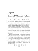
We can plot the res ults of a typical game on a graph, where the horizontal axis
represents the number of steps and the vertical axis represents the difference

between the number of stars and the number of circles that have been turned
up. A typical game is shown in Figure 6.6. In this particular game, the order
in which the cards were turned up is (C, S, S, S, S, C, C, S, S, C). Thus, in this
particular game, there were six stars and four circles in the deck. This means,
in particular, that every game played with this deck would have a graph which
ends at the point (10, 2). We define the line L to be the horizontal line which
goes through the ending point on the graph (so its vertical coordinate is just
the difference between the number of stars and circles in the deck).
(a) Show that, when the random walk is below the line L, the player guesses
right when the graph goes up (star is turned up) and, when the walk is
above the line, the player guesses right when the walk goes down (circle
turned up). Show from this property that the subject is sure to have at
least S correc t guesses.
(b) When the walk is at a point (x, x) on the line L the number of stars and
circles remaining is the same, and so the subject tosses a coin. Show that
11
P. Diaconis and R. Grah am, “The Analysis of Sequential Experiments with Feedback to Sub-
jects,” Annals of Statistics, vol. 9 (1981), pp. 3– 23.
252 CHAPTER 6. EXPECTED VALUE AND VARIANCE
2
1
1 2 3 4 5
6 7 8 9
10
(10,2)
L
Figure 6.6: Random walk for ESP.
the probability that the walk reaches (x, x) is

S

x

C
x


S+C
2x

.
Hint: The outcomes of 2x cards is a hypergeometric distribution (see
Section 5.1).
(c) Using the results of (a) and (b) show that the expected number of correct
guesses under intelligent guessing is
S +
C

x=1
1
2

S
x

C
x


S+C
2x


.
27 It has been said
12
that a Dr. B. Muriel Bristol declined a cup of tea stating
that she preferred a cup into which milk had been poured first. The famous
statistician R. A. Fisher carried out a test to see if she could tell whether milk
was put in before or after the tea. Assume that for the test Dr. Bristol was
given eight cups of tea—four in which the milk was put in before the tea and
four in which the milk was put in after the tea.
(a) What is the expected number of correct guesses the lady would make if
she had no information after each test and was just guessing?
(b) Using the result of Exercise 26 find the expected number of correct
guesses if she was told the result of each guess and used an optimal
guessing strategy.
28 In a popular computer game the computer picks an integer from 1 to n at
random. The player is given k chances to guess the number. After each guess
the computer responds “correct,” “too small,” or “too big.”
12
J. F. Box, R. A. Fisher, The Life of a Scientist (New York: John Wiley and Sons, 1978).
6.1. EXPECTED VALUE 253
(a) Show that if n ≤ 2
k
−1, then there is a strategy that guarantees you will
correctly guess the number in k tries.
(b) Show that if n ≥ 2
k
−1, there is a strategy that assures you of identifying
one of 2
k

− 1 numbers and hence gives a probability of (2
k
− 1)/n of
winning. Why is this an optimal strategy? Illustrate your result in
terms of the case n = 9 and k = 3.
29 In the casino game of blackjack the dealer is dealt two cards, one face up and
one face down, and each player is dealt two cards, both face down. If the
dealer is showing an ace the player can look at his down cards and then make
a bet called an insurance bet. (Expert players will recognize why it is called
insurance.) If you make this bet you will win the bet if the dealer’s second
card is a ten card: namely, a ten, jack, queen, or king. If you win, you are
paid twice your insurance bet; otherwise you lose this bet. Show that, if the
only cards you can see are the dealer’s ace and your two cards and if your
cards are not ten cards, then the insurance bet is an unfavorable bet. Show,
however, that if you are playing two hands simultaneously, and you have no
ten cards, then it is a favorable bet. (Thorp
13
has shown that the game of
blackjack is favorable to the player if he or she can keep good enough track
of the cards that have been played.)
30 Assume that, every time you buy a box of Wheaties, you receive a picture of
one of the n players for the New York Yankees (see Exercise 3.2.34). Let X
k
be the number of additional boxes you have to buy, after you have obtained
k −1 different pictures, in order to obtain the next new picture. Thus X
1
= 1,
X
2
is the number of boxes bought after this to obtain a picture different from

the first pictured obtained, and so forth.
(a) Show that X
k
has a geometric distribution with p = (n −k + 1)/n.
(b) Simulate the experiment for a team with 26 players (25 would be more
accurate but we want an even number). Carry out a number of simula-
tions and estimate the expected time required to get the first 13 players
and the expected time to get the second 13. How do these expectations
compare?
(c) Show that, if there are 2n players, the expected time to get the first half
of the players is
2n

1
2n
+
1
2n − 1
+ ···+
1
n + 1

,
and the expected time to get the second half is
2n

1
n
+
1

n − 1
+ ···+ 1

.
13
E. Thorp, Beat the Dealer (New York: Random House, 1962).
254 CHAPTER 6. EXPECTED VALUE AND VARIANCE
(d) In Example 6.11 we stated that
1 +
1
2
+
1
3
+ ···+
1
n
∼ log n + .5772 +
1
2n
.
Use this to estimate the expression in (c). Compare these estimates with
the exact values and also with your estimates obtained by simulation for
the case n = 26.
*31 (Feller
14
) A large number, N, of people are subjected to a blood test. This
can be administered in two ways: (1) Each person can be tested separately,
in this case N test are required, (2) the blood samples of k persons can be
pooled and analyzed together. If this test is negative, this one test suffices

for the k people. If the test is positive, each of the k persons must b e tested
separately, and in all, k + 1 tests are required for the k people. Assume that
the probability p that a test is positive is the same for all people and that
these events are independent.
(a) Find the probability that the test for a pooled sample of k people will
be positive.
(b) What is the expected value of the number X of tests necessary under
plan (2)? (Assume that N is divisible by k.)
(c) For small p, show that the value of k which will minimize the exp e cte d
number of tests under the second plan is approximately 1/
√
p.
32 Write a program to add random numbers chosen from [0, 1] until the first
time the sum is greater than one. Have your program repeat this experiment
a number of times to estimate the expected number of selections necessary
in order that the sum of the chosen numbers first exceeds 1. On the basis of
your experiments, what is your estimate for this number?
*33 The following related discrete problem also gives a good clue for the answer
to Exercise 32. Randomly select with replacement t
1
, t
2
, . . . , t
r
from the set
(1/n, 2/n, . . . , n/n). Let X be the smallest value of r satisfying
t
1
+ t
2

+ ···+ t
r
> 1 .
Then E(X) = (1 + 1/n)
n
. To prove this, we can just as well choose t
1
, t
2
,
. . . , t
r
randomly with replacement from the set (1, 2, . . . , n) and let X be the
smallest value of r for which
t
1
+ t
2
+ ···+ t
r
> n .
(a) Use Exercise 3.2.36 to show that
P (X ≥ j + 1) =

n
j


1
n


j
.
14
W. Feller, Introduction to Probability Theory and Its Applications, 3rd ed., vol. 1 (New York:
John Wiley and Sons, 1968), p. 240.
6.1. EXPECTED VALUE 255
(b) Show that
E(X) =
n

j=0
P (X ≥ j + 1) .
(c) From these two facts, find an expression for E(X). This proof is due to
Harris Schultz.
15
*34 (Banach’s Matchbox
16
) A man carries in each of his two front pockets a box
of matches originally containing N matches. Whenever he needs a match,
he choos es a pocket at random and removes one from that box. One day he
reaches into a pocket and finds the box empty.
(a) Let p
r
denote the probability that the other pocket contains r matches.
Define a sequence of counter random variables as follows: Let X
i
= 1 if
the ith draw is from the left pocket, and 0 if it is from the right p ocket.
Interpret p

r
in terms of S
n
= X
1
+ X
2
+ ··· + X
n
. Find a binomial
expression for p
r
.
(b) Write a computer program to compute the p
r
, as well as the probability
that the other pocket contains at least r matches, for N = 100 and r
from 0 to 50.
(c) Show that (N −r)p
r
= (1/2)(2N + 1)p
r+1
− (1/2)(r + 1)p
r+1
.
(d) Evaluate

r
p
r

.
(e) Use (c) and (d) to determine the expectation E of the distribution {p
r
}.
(f) Use Stirling’s formula to obtain an approximation for E. How many
matches must each box contain to ensure a value of about 13 for the
expectation E? (Take π = 22/7.)
35 A coin is tossed until the first time a head turns up. If this occurs on the nth
toss and n is odd you win 2
n
/n, but if n is even then you lose 2
n
/n. Then if
your expected winnings exist they are given by the convergent series
1 −
1
2
+
1
3
−
1
4
+ ···
called the alternating harmonic series. It is tempting to say that this should
be the expecte d value of the experiment. Show that if we were to do this, the
expected value of an experiment would depend upon the order in which the
outcomes are listed.
36 Suppose we have an urn containing c yellow balls and d green balls. We draw
k balls, without replacement, from the urn. Find the expected number of

yellow balls drawn. Hint: Write the number of yellow balls drawn as the sum
of c random variables.
15
H. Schultz, “An Expected Value Problem,” Two-Year Mathematics Journal, vol. 10, no. 4
(1979), pp. 277–78.
16
W. Feller, Introduction to Probability Theory, vol. 1, p. 166.
256 CHAPTER 6. EXPECTED VALUE AND VARIANCE
37 The reader is referred to Example 6.13 for an explanation of the various op-
tions available in Monte Carlo roulette.
(a) Compute the expected winnings of a 1 franc bet on red under option (a).
(b) Repeat part (a) for option (b).
(c) Compare the expected winnings for all three options.
*38 (from Pittel
17
) Telephone books, n in number, are kept in a stack. The
probability that the b ook numbered i (where 1 ≤ i ≤ n) is consulted for a
given phone call is p
i
> 0, where the p
i
’s sum to 1. After a b ook is used,
it is placed at the top of the stack. Assume that the calls are independent
and evenly spaced, and that the system has been employed indefinitely far
into the past. Let d
i
be the average depth of book i in the stack. Show that
d
i
≤ d

j
whenever p
i
≥ p
j
. Thus, on the average, the more p opular books
have a tendency to be closer to the top of the stack. Hint: Let p
ij
denote the
probability that book i is above book j. Show that p
ij
= p
ij
(1 − p
j
) + p
ji
p
i
.
*39 (from Propp
18
) In the previous problem, let P be the probability that at the
present time, each book is in its proper place, i.e., book i is ith from the top.
Find a formula for P in terms of the p
i
’s. In addition, find the least upper
bound on P , if the p
i
’s are allowed to vary. Hint: First find the probability

that book 1 is in the right place. Then find the probability that book 2 is in
the right place, given that book 1 is in the right place. Continue.
*40 (from H. Shultz and B. Leonard
19
) A sequence of random numbers in [0, 1)
is generated until the sequence is no longer monotone increasing. The num-
bers are chosen according to the uniform distribution. What is the expected
length of the sequence? (In calculating the length, the term that destroys
monotonicity is included.) Hint: Let a
1
, a
2
, . . . be the sequence and let X
denote the length of the sequence. Then
P (X > k) = P(a
1
< a
2
< ··· < a
k
) ,
and the probability on the right-hand side is easy to calculate. Furthermore,
one can show that
E(X) = 1 + P (X > 1) + P (X > 2) + ··· .
41 Let T be the random variable that counts the number of 2-unshuffles per-
formed on an n-card deck until all of the labels on the cards are distinct. This
random variable was discussed in Section 3.3. Using Equation 3.4 in that
section, together with the formula
E(T ) =
∞


s=0
P (T > s)
17
B. Pittel, Probl em #1195, Mathematics Magazine, vol. 58, no. 3 (May 1985), pg. 183.
18
J. Propp, Problem #1159, Mathematics Magazine vol. 57, no. 1 (Feb. 1984), pg. 50.
19
H. Shultz and B. Leonard, “Unexpected Occurrences of the Number e,” Mathematics Magazine
vol. 62, no. 4 (October, 1989), pp. 269-271.
6.2. VARIANCE OF DISCRETE RANDOM VARIABLES 257
that was proved in Exercise 33, show that
E(T ) =
∞

s=0

1 −

2
s
n

n!
2
sn

.
Show that for n = 52, this expression is approximately equal to 11.7. (As was
stated in Chapter 3, this means that on the average, almost 12 riffle shuffles of

a 52-card deck are required in order for the pro c ess to be considered random.)
6.2 Variance of Discrete Random Variables
The usefulness of the expected value as a prediction for the outcome of an ex-
periment is increased when the outcome is not likely to deviate too much from the
expected value. In this section we shall introduce a measure of this deviation, called
the variance.
Variance
Definition 6.3 Let X be a numerically valued random variable with expected value
µ = E(X). Then the variance of X, denoted by V (X), is
V (X) = E((X −µ)
2
) .
✷
Note that, by Theorem 6.1, V (X) is given by
V (X) =

x
(x − µ)
2
m(x) , (6.1)
where m is the distribution function of X.
Standard Deviation
The standard deviation of X, denoted by D(X), is D(X) =

V (X). We often
write σ for D(X) and σ
2
for V (X).
Example 6.17 Consider one roll of a die. Let X be the number that turns up. To
find V (X), we must first find the expected value of X. This is

µ = E(X) = 1

1
6

+ 2

1
6

+ 3

1
6

+ 4

1
6

+ 5

1
6

+ 6

1
6


=
7
2
.
To find the variance of X, we form the new random variable (X − µ)
2
and
compute its expectation. We can easily do this using the following table.
258 CHAPTER 6. EXPECTED VALUE AND VARIANCE
x m(x) (x − 7/2)
2
1 1/6 25/4
2 1/6 9/4
3 1/6 1/4
4 1/6 1/4
5 1/6 9/4
6 1/6 25/4
Table 6.6: Variance calculation.
From this table we find E((X −µ)
2
) is
V (X) =
1
6

25
4
+
9
4

+
1
4
+
1
4
+
9
4
+
25
4

=
35
12
,
and the standard deviation D(X) =

35/12 ≈ 1.707. ✷
Calculation of Variance
We next prove a theorem that gives us a useful alternative form for computing the
variance.
Theorem 6.6 If X is any random variable with E(X) = µ, then
V (X) = E(X
2
) − µ
2
.
Proof. We have

V (X) = E((X −µ)
2
) = E(X
2
− 2µX + µ
2
)
= E(X
2
) − 2µE(X) + µ
2
= E(X
2
) − µ
2
.
✷
Using Theorem 6.6, we can compute the variance of the outcome of a roll of a
die by first computing
E(X
2
) = 1

1
6

+ 4

1
6


+ 9

1
6

+ 16

1
6

+ 25

1
6

+ 36

1
6

=
91
6
,
and,
V (X) = E(X
2
) − µ
2

=
91
6
−

7
2

2
=
35
12
,
in agreement with the value obtained directly from the definition of V (X).
6.2. VARIANCE OF DISCRETE RANDOM VARIABLES 259
Properties of Variance
The variance has properties very different from those of the expectation. If c is any
constant, E(cX) = cE(X) and E(X + c) = E(X) + c. These two statements imply
that the expectation is a linear function. However, the variance is not linear, as
seen in the next theorem.
Theorem 6.7 If X is any random variable and c is any constant, then
V (cX) = c
2
V (X)
and
V (X + c) = V (X) .
Proof. Let µ = E(X). Then E(cX) = cµ, and
V (cX) = E((cX −cµ)
2
) = E(c

2
(X −µ)
2
)
= c
2
E((X −µ)
2
) = c
2
V (X) .
To prove the second asse rtion, we note that, to compute V (X + c), we would
replace x by x+c and µ by µ+c in Equation 6.1. Then the c’s would cancel, leaving
V (X). ✷
We turn now to some general properties of the variance. Recall that if X and Y
are any two random variables, E(X+Y ) = E(X)+E(Y ). This is not always true for
the case of the variance. For example, let X b e a random variable with V (X) = 0,
and define Y = −X. Then V (X) = V (Y ), so that V (X) + V (Y ) = 2V (X). But
X + Y is always 0 and hence has variance 0. Thus V (X + Y ) = V (X) + V (Y ).
In the important case of mutually independent random variables, however, the
variance of the sum is the sum of the variances.
Theorem 6.8 Let X and Y be two independent random variables. Then
V (X + Y ) = V (X) + V (Y ) .
Proof. Let E(X) = a and E(Y ) = b. Then
V (X + Y ) = E((X + Y )
2
) − (a + b)
2
= E(X
2

) + 2E(XY ) + E(Y
2
) − a
2
− 2ab −b
2
.
Since X and Y are independent, E(XY ) = E(X)E(Y ) = ab. Thus,
V (X + Y ) = E(X
2
) − a
2
+ E(Y
2
) − b
2
= V (X) + V (Y ) .
✷
260 CHAPTER 6. EXPECTED VALUE AND VARIANCE
It is easy to extend this proof, by mathematical induction, to show that the
variance of the sum of any number of mutually independent random variables is the
sum of the individual variances. Thus we have the following theorem.
Theorem 6.9 Let X
1
, X
2
, . . . , X
n
be an independent trials process with E(X
j

) =
µ and V (X
j
) = σ
2
. Let
S
n
= X
1
+ X
2
+ ···+ X
n
be the sum, and
A
n
=
S
n
n
be the average. Then
E(S
n
) = nµ ,
V (S
n
) = nσ
2
,

σ(S
n
) = σ
√
n ,
E(A
n
) = µ ,
V (A
n
) =
σ
2
n
,
σ(A
n
) =
σ
√
n
.
Proof. Since all the random variables X
j
have the same expected value, we have
E(S
n
) = E(X
1
) + ··· + E(X

n
) = nµ ,
V (S
n
) = V (X
1
) + ··· + V (X
n
) = nσ
2
,
and
σ(S
n
) = σ
√
n .
We have seen that, if we multiply a random variable X with mean µ and variance
σ
2
by a constant c, the new random variable has expected value cµ and variance
c
2
σ
2
. Thus,
E(A
n
) = E


S
n
n

=
nµ
n
= µ ,
and
V (A
n
) = V

S
n
n

=
V (S
n
)
n
2
=
nσ
2
n
2
=
σ

2
n
.
Finally, the standard deviation of A
n
is given by
σ(A
n
) =
σ
√
n
.
✷
6.2. VARIANCE OF DISCRETE RANDOM VARIABLES 261
1 2
3
4
5
6
0
0.1
0.2
0.3
0.4
0.5
0.6
2
2.5 3 3.5
4

4.5
5
0
0.5
1
1.5
2
n = 10 n = 100
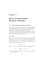
Figure 6.7: Empirical distribution of A
n
.
The last equation in the above theorem implies that in an independent trials
process, if the individual summands have finite variance, then the standard devi-
ation of the average goes to 0 as n → ∞. Since the standard deviation tells us
something about the spread of the distribution around the mean, we see that for
large values of n, the value of A
n
is usually very close to the mean of A
n
, which
equals µ, as shown above. This statement is made precise in Chapter 8, where it
is called the Law of Large Numbers. For example, let X represent the roll of a fair
die. In Figure 6.7, we show the distribution of a random variable A
n
corresponding
to X, for n = 10 and n = 100.
Example 6.18 Consider n rolls of a die. We have seen that, if X
j
is the outcome
if the jth roll, then E(X

j
) = 7/2 and V (X
j
) = 35/12. Thus, if S
n
is the sum of the
outcomes, and A
n
= S
n
/n is the average of the outcomes, we have E(A
n
) = 7/2 and
V (A
n
) = (35/12)/n. Therefore, as n increases, the expected value of the average
remains constant, but the variance tends to 0. If the variance is a measure of the
expected deviation from the mean this would indicate that, for large n, we can
expect the average to be very near the expected value. This is in fact the case, and
we shall justify it in Chapter 8. ✷
Bernoulli Trials
Consider next the general B ernoulli trials process. As usual, we let X
j
= 1 if the
jth outcome is a success and 0 if it is a failure. If p is the probability of a success,
and q = 1 − p, then
E(X
j
) = 0q + 1p = p ,
E(X

2
j
) = 0
2
q + 1
2
p = p ,
and
V (X
j
) = E(X
2
j
) − (E(X
j
))
2
= p −p
2
= pq .
Thus, for Bernoulli trials, if S
n
= X
1
+X
2
+···+ X
n
is the number of successes,
then E(S

n
) = np, V (S
n
) = npq, and D(S
n
) =
√
npq. If A
n
= S
n
/n is the average
number of successes, then E(A
n
) = p, V (A
n
) = pq/n, and D(A
n
) =

pq/n. We
see that the expected proportion of successes remains p and the variance tends to 0.
262 CHAPTER 6. EXPECTED VALUE AND VARIANCE
This suggests that the frequency interpretation of probability is a correct one. We
shall make this more precise in Chapter 8.
Example 6.19 Let T denote the number of trials until the first success in a
Bernoulli trials process. Then T is geometrically distributed. What is the vari-
ance of T ? In Example 4.15, we saw that
m
T

=

1 2 3 ···
p qp q
2
p ···

.
In Example 6.4, we showed that
E(T ) = 1/p .
Thus,
V (T ) = E(T
2
) − 1/p
2
,
so we need only find
E(T
2
) = 1p + 4qp + 9q
2
p + ···
= p(1 + 4q + 9q
2
+ ···) .
To evaluate this sum, we start again with
1 + x + x
2
+ ··· =
1

1 − x
.
Differentiating, we obtain
1 + 2x + 3x
2
+ ··· =
1
(1 − x)
2
.
Multiplying by x,
x + 2x
2
+ 3x
3
+ ··· =
x
(1 − x)
2
.
Differentiating again gives
1 + 4x + 9x
2
+ ··· =
1 + x
(1 − x)
3
.
Thus,
E(T

2
) = p
1 + q
(1 − q)
3
=
1 + q
p
2
and
V (T ) = E(T
2
) − (E(T ))
2
=
1 + q
p
2
−
1
p
2
=
q
p
2
.
For example, the variance for the number of tosse s of a coin until the first
head turns up is (1/2)/(1/2)
2

= 2. The variance for the number of rolls of a
die until the first six turns up is (5/6)/(1/6)
2
= 30. Note that, as p decreases, the
variance increases rapidly. This corresponds to the increased spread of the geometric
distribution as p decreases (noted in Figure 5.1). ✷
6.2. VARIANCE OF DISCRETE RANDOM VARIABLES 263
Poisson Distribution
Just as in the case of expected values, it is easy to guess the variance of the Poisson
distribution with parameter λ. We recall that the variance of a binomial distribution
with parameters n and p equals npq. We also recall that the Poisson distribution
could be obtained as a limit of binomial distributions, if n goes to ∞ and p goes
to 0 in such a way that their product is kept fixed at the value λ. In this case,
npq = λq approaches λ, since q goes to 1. So, given a Poisson distribution with
parameter λ, we should guess that its variance is λ. The reader is asked to show
this in Exercise 29.
Exercises
1 A number is chosen at random from the set S = {−1, 0, 1}. Let X be the
number chosen. Find the expected value, variance, and standard deviation of
X.
2 A random variable X has the distribution
p
X
=

0 1 2 4
1/3 1/3 1/6 1/6

.
Find the expected value, variance, and standard deviation of X.

3 You place a 1-dollar bet on the number 17 at Las Vegas, and your friend
places a 1-dollar bet on black (see Exercises 1.1.6 and 1.1.7). Let X be your
winnings and Y be her winnings. Compare E(X), E(Y ), and V (X), V (Y ).
What do these computations tell you ab out the nature of your winnings if
you and your friend make a se quence of bets, with you betting each time on
a number and your friend betting on a color?
4 X is a random variable with E(X) = 100 and V (X) = 15. Find
(a) E(X
2
).
(b) E(3X + 10).
(c) E(−X).
(d) V (−X).
(e) D(−X).
5 In a certain manufacturing process, the (Fahrenheit) temperature never varies
by more than 2
◦
from 62
◦
. The temperature is, in fact, a random variable F
with distribution
P
F
=

60 61 62 63 64
1/10 2/10 4/10 2/10 1/10

.
(a) Find E(F ) and V (F ).

(b) Define T = F − 62. Find E(T ) and V (T ), and compare these answers
with those in part (a).
264 CHAPTER 6. EXPECTED VALUE AND VARIANCE
(c) It is decided to report the temperature readings on a Celsius scale, that
is, C = (5/9)(F − 32). What is the expected value and variance for the
readings now?
6 Write a computer program to calculate the mean and variance of a distribution
which you specify as data. Use the program to compare the variances for the
following densities, both having expected value 0:
p
X
=

−2 −1 0 1 2
3/11 2/11 1/11 2/11 3/11

;
p
Y
=

−2 −1 0 1 2
1/11 2/11 5/11 2/11 1/11

.
7 A coin is tossed three times. Let X be the number of heads that turn up.
Find V (X) and D(X).
8 A random sample of 2400 people are asked if they favor a government pro-
posal to develop new nuclear power plants. If 40 percent of the people in the
country are in favor of this proposal, find the expected value and the stan-

dard deviation for the number S
2400
of people in the sample who favored the
prop os al.
9 A die is loaded so that the probability of a face coming up is proportional to
the numbe r on that face. The die is rolled with outcome X. Find V (X) and
D(X).
10 Prove the following facts about the standard deviation.
(a) D(X + c) = D(X).
(b) D(cX) = |c|D(X).
11 A number is chosen at random from the integers 1, 2, 3, . . . , n. Let X be the
number chosen. Show that E(X) = (n + 1)/2 and V (X) = (n −1)(n + 1)/12.
Hint: The following identity may be useful:
1
2
+ 2
2
+ ···+ n
2
=
(n)(n + 1)(2n + 1)
6
.
12 Let X be a random variable with µ = E(X) and σ
2
= V (X). Define X
∗
=
(X−µ)/σ. The random variable X
∗

is called the standardized random variable
associated with X. Show that this standardized random variable has expected
value 0 and variance 1.
13 Peter and Paul play Heads or Tails (see Example 1.4). Let W
n
be Peter’s
winnings after n matches. Show that E(W
n
) = 0 and V (W
n
) = n.
14 Find the expected value and the variance for the number of boys and the
number of girls in a royal family that has children until there is a boy or until
there are three children, whichever comes first.
6.2. VARIANCE OF DISCRETE RANDOM VARIABLES 265
15 Suppose that n people have their hats returned at random. Let X
i
= 1 if the
ith person gets his or her own hat back and 0 otherwise. Let S
n
=

n
i=1
X
i
.
Then S
n
is the total number of people who get their own hats back. Show

that
(a) E(X
2
i
) = 1/n.
(b) E(X
i
· X
j
) = 1/n(n −1) for i = j.
(c) E(S
2
n
) = 2 (using (a) and (b)).
(d) V (S
n
) = 1.
16 Let S
n
be the number of successes in n independent trials. Use the program
BinomialProbabilities (Section 3.2) to compute, for given n, p, and j, the
probability
P (−j
√
npq < S
n
− np < j
√
npq) .
(a) Let p = .5, and compute this probability for j = 1, 2, 3 and n = 10, 30, 50.

Do the same for p = .2.
(b) Show that the standardized random variable S
∗
n
= (S
n
− np)/
√
npq has
expected value 0 and variance 1. What do your results from (a) tell you
about this standardized quantity S
∗
n
?
17 Let X be the outcome of a chance experiment with E(X) = µ and V (X) =
σ
2
. When µ and σ
2
are unknown, the statistician often estimates them by
repeating the experiment n times with outcomes x
1
, x
2
, . . . , x
n
, estimating
µ by the sample mean
¯x =
1

n
n

i=1
x
i
,
and σ
2
by the sample variance
s
2
=
1
n
n

i=1
(x
i
− ¯x)
2
.
Then s is the sample standard deviation. These formulas should remind the
reader of the definitions of the theoretical mean and variance. (Many statisti-
cians define the sample variance with the coefficient 1/n replaced by 1/(n−1).
If this alternative definition is used, the expected value of s
2
is equal to σ
2

.
See Exercise 18, part (d).)
Write a computer program that will roll a die n times and compute the sample
mean and sample variance. Repeat this experiment several times for n = 10
and n = 1000. How well do the sample mean and sample variance estimate
the true mean 7/2 and variance 35/12?
18 Show that, for the sample mean ¯x and sample variance s
2
as defined in Exer-
cise 17,
(a) E(¯x) = µ.
266 CHAPTER 6. EXPECTED VALUE AND VARIANCE
(b) E

(¯x − µ)
2

= σ
2
/n.
(c) E(s
2
) =
n−1
n
σ
2
. Hint: For (c) write
n


i=1
(x
i
− ¯x)
2
=
n

i=1

(x
i
− µ) −(¯x − µ)

2
=
n

i=1
(x
i
− µ)
2
− 2(¯x −µ)
n

i=1
(x
i
− µ) + n(¯x − µ)

2
=
n

i=1
(x
i
− µ)
2
− n(¯x −µ)
2
,
and take expectations of both sides, using part (b) when necessary.
(d) Show that if, in the definition of s
2
in Exercise 17, we replace the co e ffi-
cient 1/n by the coefficient 1/(n −1), then E(s
2
) = σ
2
. (This shows why
many statisticians use the coefficient 1/(n − 1). The number s
2
is used
to estimate the unknown quantity σ
2
. If an estimator has an average
value which equals the quantity being estimated, then the estimator is
said to be unbiased. Thus, the stateme nt E(s
2

) = σ
2
says that s
2
is an
unbiased estimator of σ
2
.)
19 Let X be a random variable taking on values a
1
, a
2
, . . . , a
r
with probabilities
p
1
, p
2
, . . . , p
r
and with E(X) = µ. Define the spread of X as follows:
¯σ =
r

i=1
|a
i
− µ|p
i

.
This, like the standard deviation, is a way to quantify the amount that a
random variable is spread out around its mean. Recall that the variance of a
sum of mutually independent random variables is the sum of the individual
variances. The square of the spread corresponds to the variance in a manner
similar to the correspondence between the spread and the standard deviation.
Show by an example that it is not necessarily true that the square of the
spread of the sum of two independent random variables is the sum of the
squares of the individual spreads.
20 We have two instruments that measure the distance between two points. The
measurements given by the two instruments are random variables X
1
and
X
2
that are independent with E(X
1
) = E(X
2
) = µ, where µ is the true
distance. From experience with these instruments, we know the values of the
variances σ
2
1
and σ
2
2
. These variances are not necessarily the same. From two
measurements, we estimate µ by the weighted average ¯µ = wX
1

+ (1 −w)X
2
.
Here w is chosen in [0, 1] to minimize the variance of ¯µ.
(a) What is E(¯µ)?
(b) How should w be chosen in [0, 1] to minimize the variance of ¯µ?
6.2. VARIANCE OF DISCRETE RANDOM VARIABLES 267
21 Let X be a random variable with E(X) = µ and V (X) = σ
2
. Show that the
function f(x) defined by
f(x) =

ω
(X(ω) −x)
2
p(ω)
has its minimum value when x = µ.
22 Let X and Y be two random variables defined on the finite sample space Ω.
Assume that X, Y , X + Y , and X −Y all have the same distribution. Prove
that P (X = Y = 0) = 1.
23 If X and Y are any two random variables, then the covariance of X and Y is
defined by Cov(X, Y ) = E((X −E(X))(Y −E(Y ))). Note that Cov(X, X) =
V (X). Show that, if X and Y are independent, then Cov(X, Y ) = 0; and
show, by an example, that we can have Cov(X, Y ) = 0 and X and Y not
independent.
*24 A professor wishes to make up a true-false exam with n questions. She assumes
that she can design the problems in such a way that a student will answer
the jth problem correctly with probability p
j

, and that the answers to the
various problems may be considered independent experiments. Let S
n
be the
number of problems that a student will get correct. The professor wishes to
choose p
j
so that E(S
n
) = .7n and so that the variance of S
n
is as large as
possible. Show that, to achieve this, she should choose p
j
= .7 for all j; that
is, she should make all the problems have the same difficulty.
25 (Lamperti
20
) An urn contains exactly 5000 balls, of which an unknown number
X are white and the rest red, where X is a random variable with a probability
distribution on the integers 0, 1, 2, . . . , 5000.
(a) Suppose we know that E(X) = µ. Show that this is enough to allow us
to calculate the probability that a ball drawn at random from the urn
will be white. What is this probability?
(b) We draw a ball from the urn, examine its color, re place it, and then
draw another. Under what conditions, if any, are the results of the two
drawings independent; that is, does
P (white, white) = P(white)
2
?

(c) Suppose the variance of X is σ
2
. What is the probability of drawing two
white balls in part (b)?
26 For a sequence of Bernoulli trials, let X
1
be the number of trials until the first
success. For j ≥ 2, let X
j
be the number of trials after the (j −1)st success
until the jth success. It can be shown that X
1
, X
2
, . . . is an independent trials
process.
20
Private communication.
268 CHAPTER 6. EXPECTED VALUE AND VARIANCE
(a) What is the common distribution, expected value, and variance for X
j
?
(b) Let T
n
= X
1
+ X
2
+ ···+ X
n

. Then T
n
is the time until the nth success.
Find E(T
n
) and V (T
n
).
(c) Use the results of (b) to find the expected value and variance for the
number of tosses of a coin until the nth occurrence of a head.
27 Referring to Exercise 6.1.30, find the variance for the number of boxes of
Wheaties b ought before getting half of the players’ pictures and the variance
for the number of additional boxes needed to get the second half of the players’
pictures.
28 In Example 5.3, assume that the book in question has 1000 pages. Le t X be
the number of pages with no mistakes. Show that E(X) = 905 and V (X) =
86. Using these results, show that the probability is ≤ .05 that there will be
more than 924 pages without errors or fewer than 866 pages without errors.
29 Let X be Poisson distributed with parameter λ. Show that V (X) = λ.
6.3 Continuous Random Variables
In this section we consider the properties of the expected value and the variance
of a continuous random variable. These quantities are defined just as for discrete
random variables and share the same properties.
Expected Value
Definition 6.4 Let X be a real-valued random variable with density function f (x).
The expected value µ = E(X) is defined by
µ = E(X) =

+∞
−∞

xf(x) dx ,
provided the integral

+∞
−∞
|x|f(x) dx
is finite. ✷
The reader should compare this definition with the corresponding one for discrete
random variables in Section 6.1. Intuitively, we can interpret E(X), as we did in
the previous sections, as the value that we should expect to obtain if we perform a
large number of independent experiments and average the resulting values of X.
We can summarize the properties of E(X) as follows (cf. Theorem 6.2).
6.3. CONTINUOUS RANDOM VARIABLES 269
Theorem 6.10 If X and Y are real-valued random variables and c is any constant,
then
E(X + Y ) = E(X) + E(Y ) ,
E(cX) = cE(X) .
The proof is very similar to the proof of Theorem 6.2, and we omit it. ✷
More generally, if X
1
, X
2
, . . . , X
n
are n real-valued random variables, and c
1
, c
2
,
. . . , c

n
are n constants, then
E(c
1
X
1
+ c
2
X
2
+ ···+ c
n
X
n
) = c
1
E(X
1
) + c
2
E(X
2
) + ··· + c
n
E(X
n
) .
Example 6.20 Let X be uniformly distributed on the interval [0, 1]. Then
E(X) =


1
0
x dx = 1/2 .
It follows that if we choose a large number N of random numbers from [0, 1] and take
the average, then we can expect that this average should be close to the expected
value of 1/2. ✷
Example 6.21 Let Z = (x, y) denote a point chosen uniformly and randomly from
the unit disk, as in the dart game in Example 2.8 and let X = (x
2
+ y
2
)
1/2
be the
distance from Z to the center of the disk. The density function of X can easily be
shown to equal f (x) = 2x, so by the definition of expected value,
E(X) =

1
0
xf(x) dx
=

1
0
x(2x) dx
=
2
3
.

✷
Example 6.22 In the example of the couple meeting at the Inn (Example 2.16),
each person arrives at a time which is uniformly distributed between 5:00 and 6:00
PM. The random variable Z under consideration is the length of time the first
person has to wait until the second one arrives. It was shown that
f
Z
(z) = 2(1 − z) ,
for 0 ≤ z ≤ 1. Hence,
E(Z) =

1
0
zf
Z
(z) dz
270 CHAPTER 6. EXPECTED VALUE AND VARIANCE
=

1
0
2z(1 −z) dz
=

z
2
−
2
3
z

3

1
0
=
1
3
.
✷
Expectation of a Function of a Random Variable
Supp ose that X is a real-valued random variable and φ(x) is a continuous function
from R to R. The following theorem is the continuous analogue of Theorem 6.1.
Theorem 6.11 If X is a real-valued random variable and if φ : R → R is a
continuous real-valued function with domain [a, b], then
E(φ(X)) =

+∞
−∞
φ(x)f
X
(x) dx ,
provided the integral exists. ✷
For a proof of this theorem, see Ross.
21
Expectation of the Product of Two Random Variables
In general, it is not true that E(XY ) = E(X)E(Y ), since the integral of a product is
not the product of integrals. But if X and Y are independent, then the expectations
multiply.
Theorem 6.12 Let X and Y be independent real-valued continuous random vari-
ables with finite expected values. Then we have

E(XY ) = E(X)E(Y ) .
Proof. We will prove this only in the case that the ranges of X and Y are c ontained
in the intervals [a, b] and [c, d], respectively. Let the density functions of X and Y
be denoted by f
X
(x) and f
Y
(y), respectively. Since X and Y are independent, the
joint density function of X and Y is the product of the individual density functions.
Hence
E(XY ) =

b
a

d
c
xyf
X
(x)f
Y
(y) dy dx
=

b
a
xf
X
(x) dx


d
c
yf
Y
(y) dy
= E(X)E(Y ) .
The proof in the general case involves using sequences of bounded random vari-
ables that approach X and Y , and is somewhat technical, so we will omit it. ✷
21
S. Ross, A First Course in Probability, (New York: Macmillan, 1984), pgs. 241-245.
6.3. CONTINUOUS RANDOM VARIABLES 271
In the same way, one can show that if X
1
, X
2
, . . . , X
n
are n mutually indepen-
dent real-valued random variables, then
E(X
1
X
2
···X
n
) = E(X
1
) E(X
2
) ··· E(X

n
) .
Example 6.23 Let Z = (X , Y ) be a point chosen at random in the unit square.
Let A = X
2
and B = Y
2
. Then Theorem 4.3 implies that A and B are independent.
Using Theorem 6.11, the expectations of A and B are easy to calculate:
E(A) = E(B) =

1
0
x
2
dx
=
1
3
.
Using Theorem 6.12, the expectation of AB is just the product of E(A) and E(B),
or 1/9. The usefulness of this theorem is demonstrated by noting that it is quite a
bit more difficult to calculate E(AB) from the definition of expectation. One finds
that the density function of AB is
f
AB
(t) =
−log(t)
4
√

t
,
so
E(AB) =

1
0
tf
AB
(t) dt
=
1
9
.
✷
Example 6.24 Again let Z = (X, Y ) be a point chosen at random in the unit
square, and let W = X + Y . Then Y and W are not independent, and we have
E(Y ) =
1
2
,
E(W ) = 1 ,
E(Y W ) = E(XY + Y
2
) = E(X)E(Y ) +
1
3
=
7
12

= E(Y )E(W ) .
✷
We turn now to the variance.
Variance
Definition 6.5 Let X be a real-valued random variable with density function f (x).
The variance σ
2
= V (X) is defined by
σ
2
= V (X) = E((X −µ)
2
) .
✷