Advances in Robot Kinematics - Jadran Lenarcic and Bernard Roth (Eds) Part 3 ppt
Bạn đang xem bản rút gọn của tài liệu. Xem và tải ngay bản đầy đủ của tài liệu tại đây (1.73 MB, 30 trang )
d.o.f. of the chains. It is also possible to obtain chains that change G
but
not the number of d.o.f. Using again the scheme of Fig. 2, the results
From these results the schemes of Fig. 5 are obtained. Other similar
configurations can be obtained through suitable permutations of
kinematic pairs and groups.
Table 2. Modified groups and pairs in Fig. 1
Case G
1
= G
2
KP
a
= KP
b
Displacements between a
1
and b
2
d
E (planar)
X
(Schoenflies)
From E to a subset of X with 3 d.o.f.
e
Y (translating
screw)
X
(Schoenflies)
From Y to a subset of X with 3 d.o.f.
Figure 6 shows the kinematic chains resulting from the two cases d
separates the two branches of positions belonging to different groups.
Figure 6. Robots that change displacement group but not No. of d.o.f.
53
reported in Table 2 can be achieved (see Fanghella and Galletti, 1994).
and e of Table 2. The chains are drawn in their singular position that
Figure 5. Robots with E, X, Y, and R groups.
Parallel Robots that Change their Group of Motion
.
For example, in the case d, starting from the position drawn and
rotating the revolutes with horizontal axes, the robot acts as a standard
planar platform, with 3 d.o.f. Starting again from the singular position,
translations and 1 rotation). Then, the group of displacement is changed,
but the number of d.o.f. is preserved.
An analogous situation applies to case e.
A slightly different case can be derived from a further interesting
intersection group. Two Schoenflies groups X can give a group G
= X or
a group G
= U (three-dimensional translation), depending on the
relative positions of their rotation directions (see Fanghella and Galletti,
Case G
1
= G
2
KP
a
= KP
b
Displacements between a
1
and b
2
f
X
(Schoenflies)
R
From the original X (Schoenflies)
to an X (Schoenflies) with the axis
parallel to the axis of R
Since a group X with 4 d.o.f. is obtained in both branches, the platform
must have 4 legs in order to apply one driver to each leg, according to the
scheme of Fig. 7.
X
R
X
X
X
R
R
R
Figure 8 shows the resulting kinematic chain of the robot in the
singular position where the two branches merge.
Starting from this position and rotating the revolutes with horizontal
axes, the platform moves in an X group with a horizontal rotation axis,
the vertical revolutes being locked. The number of d.o.f. is 4. Starting
again from the singular position, by moving the revolutes with vertical
axes, the platform moves in an X group with a vertical rotation axis, the
horizontal revolutes resulting locked. Again the number of d.o.f. is 4. The
54
1994). Therefore, according to Fig. 2, the following chain can be derived.
Figure 7. Scheme of a 4-legs robot.
P. Fanghella, C. Galletti and E. Giannotti
by moving the revolutes with vertical axes, the platform of the robot
has a displacement that is a subset of the group X, with 3 d.o.f. (2
group of displacement is not changed, but its invariant property (rotation
axis) is changed.
X
frame
platform
X
X
R
R
R
X
X
R
X
frame
5.
The schemes of Figs. 3, 5, and 7, define kinematic structures in which
specific displacement groups are generated by sequences of bodies and
pairs. It is evident that in order to obtain the aforesaid mobility
properties, the way in which the groups GR are realized is immaterial.
For instance, it is well known that the group X can be generated by 3 non
pairs. Therefore, many different robot structures can be obtained
starting from the schemes of Figs. 3, 5, and 7.
From a practical point of view, in order to control the motion of a
kinematotropic chain in a branch it is necessary to provide a number of
drivers equal to the number of degrees of freedom of the chain in that
branch. For a complete control of the chain in all branches, it is
necessary to provide a set of drivers equal to the union of the drivers
used to control each branch. In each branch, the chain is actuated only by
the drivers associated with that branch, while other drivers become
driven; when passing through a singular position (where the number of
infinitesimal degrees of freedom grows), all drivers must act either to
maintain their position or to drive the chain to a specific branch.
Finally, it is worth noting that, in some cases, starting from the
direction orthogonal to the drawing plane leads to a branch in which the
55
Joint Modifications, Actuators and Branches
be reached. For example, for the mechanism in Fig. 6-d, a translation in the
singular positions in Figs. 4, 6 and 8, more than two branches may
Figure 8. Robot that changes the invariant of its displacement group.
Parallel Robots that Change their Group of Motion
parallel prismatic pairs and one revolute, by 3 parallel revolutes and
1 prismatic pair not normal to them, and so on. Moreover, the revolutes
KP in the chains can be substituted, in several circumstances by helical
allowed relative motion between the frame and the platform is a pure
planar translation. In the paper, for each case, the discussion is limited
to the two branches with the highest number of degrees of freedom.
6. Conclusions
Special kinematic chains, in which displacements between two bodies
can belong to different displacement groups when the chains are moved
situations arise for the displacement of the platform when the robot is
displaced continuously from one set of positions to another one: i) in 3
cases the platform can change its group of displacement and the number
degrees of freedom; ii) in 2 cases only the group of displacement is
altered; iii) in 1 case only the invariant properties of the group of
displacement are modified.
References
Angeles J. (1988), Rational Kinematics, Springer.
Fanghella P. and Galletti C. (1994), Mobility Analysis of Single-Loop Kinematic
Chains: An Algorithmic Approach Based on Displacement Groups,
Mechanism and Machine Theory, Vol. 29, pp. 1187-1204.
Galletti C. and Fanghella P. (2001), Single-Loop Kinematotropic Mechanisms,
Mechanism and Machine Theory, Vol. 36, pp. 743-761.
Gogu G. (2005), Mobility Criterion and Overconstraints of Parallel Manipulators,
Proc. of CK2005 Int. Workshop on Computational Kinematics, Cassino, Paper
22-CK2005, pp. 1-16.
Hervé J. (1978), Analyse Structurelle des Mécanismes par Groupe des
Déplacements, Mechanism and Machine Theory, Vol. 13, pp. 437-450.
Kong X. and Gosselin C. (2004), Type Synthesis of 3T1R 4-DOF Parallel
Manipulators Based on Screw Theory, IEEE Transactions on Robotics and
Automation, Vol. 20, pp. 181-190.
Kong X. and Gosselin C. (2005), Type Synthesis of 3-DOF PPR-Equivalent
Parallel Manipulators Based on Screw Theory and the Concept of Virtual
Chain, ASME J. of Mechanical Design, Vol. 127, pp. 1113-1121.
Wohlhart K. (1996), Kinematotropic Mechanisms, Recent Advances in Robot
Kinematics, (J. Lenarcic and V. Parenti Castelli, Eds.), Kluwer , pp. 359-368.
This work has been developed under a grant of
Italian MIUR
56
.
P. Fanghella, C. Galletti and E. Giannotti
by one branch to another, are the basic components we have used
for synthesizing a particular type of parallel robots. Three different
Acknowledgement
APPROXIMATING PLANAR, MORPHING
CURVES WITH RIGID-BODY LINKAGES
Andrew P. Murray
University of Dayton, Department of Mechanical & Aerospace Engineering
Dayton, OH USA
Brian M. Korte and James P. Schmiedeler
The Ohio State University, Department of Mechanical Engineering
Columbus, OH USA
&
Abstract This paper presents a procedure to synthesize planar linkages, composed
of rigid links and revolute joints, that approximate a shape change de-
fined by a set of curves. These “morphing curves” differ from each
other by a combination of rigid-body displacement and shape change.
Rigid link geometry is determined through analysis of piecewise linear
curves, and increasing the number of links improves the shape-change
approximation. The framework is applied to an open-chain example.
Keywords: Shape change, morphing structures, planar synthesis
1. Introduction
For a mechanical system whose function depends on its geometric
shape, the controlled ability to change that shape can enhance per-
formance or expand applications. Examples of adaptive or morphing
structures include antenna reflectors (Washington, 1996) and airfoils
(Bart-Smith & Risseeuw, 2003) proposed to include many smart mater-
ial actuators. Compliant mechanisms also provide a means of achieving
shape changes. Saggere & Kota, 2001 developed a synthesis procedure
for compliant four-bars that guide their flexible couplers through dis
-
crete prescribed “precision shapes” that involve both shape change and
rigid-body displacement. Lu & Kota, 2003 introduced a more general
approach using finite element analysis and a genetic algorithm to deter-
mine an optimized compliant mechanism’s topology and dimensions.
The present work introduces synthesis techniques for planar, rigid-
body mechanisms that approximate a desired shape change defined by
an arbitrary number of curves, one morphing into another. Higher load-
57
carrying capacity makes rigid-body mechanisms better suited than
J. Lenarþiþ and B. Roth (eds.), Advances in Robot Kinematics, 57 64.
© 2006 Springer. Printed in the Netherlands.
−
rigid-body mechanisms would likely require fewer actuators acting in
parallel, such as along an airfoil with changing camber. Furthermore,
actuation is not an additional development need because existing tech-
nology rather than, for example, smart material technology, is typically
used to actuate rigid-body mechanisms. With rigid links, synthesis can
a
can typically achieve larger displacements, enabling more dramatic shape
changes. This paper details a methodology for designing rigid links that
can be joined together in a chain by revolute joints to approximate the
shapes of a set of morphing curves. The methodology is applicable to
both open and closed chains, and an open-chain example is presented.
2. Rigid Link Geometry
linkage involves converting the desired curves, denoted as “design pro-
files”, into “target profiles” that are readily manipulated and compared.
The target profiles are divided into segments, and corresponding seg-
ments from all of the target profiles are used to generate the rigid links.
The key is to divide the target profiles and then generate the rigid links
so as to reduce the error in approximating the design profiles.
Design Profiles and Target Profiles. Adesignprofileisacurve
defined such that an ordered set of points on the curve and the arc length
between any two such points can be determined. The piecewise linear
curve (solid line) in Fig. 1 is a simple example of a design profile. A
set of p design profiles defines a shape change problem. Because the
change will be approximated with a rigid-body linkage, the error in the
approximation is generally smaller if all p profiles have roughly equal arc
length, though this is not an explicit requirement of the methodology.
A target profile is formed by distributing n points, separated by equal
arc lengths, along a design profile. Thus, a target profile is a piecewise
linear curve composed of the line segments connecting the ordered set of
points, and any design profile can be represented by a target profile of
two or more points. In Fig. 1, five (x, y) points generate a target profile
from the design profile defined by three (a, b) points. The target profile
includes the dashed line and does not pass through the design profile’s
second point. In this case, three points could be used to exactly represent
the design profile, but the approach is more generally applicable to any
design profile. The motivation is to convert a set of p design profiles into
target profiles all defined by n points such that corresponding points can
A.P. Murray, B.M. Korte and J.P. Schmiedeler 58
com
pliant mechanisms for applications with large applied loads. Similarly,
priori knowledge of exact external loads. Finally, rigid-body mechanisms
be purely kinematic, so the system can be modeled precisely without
The procedure for generating rigid links that compose a shape-changing
Figure 1. Three-point (a, b) design profile and five-point (x, y) target profile.
be found on each target profile. For a closed curve design profile, any
point can be deemed the first/last point, yielding a closed target profile.
Important characteristics of a target profile include the fact that its
arclengthisalwaysshorterthanthedesignprofileitrepresents. The
most significant loss of shape information occurs where the curvature is
largest for a continuous design profile or where the angle at a vertex is
smallest in magnitude for a piecewise linear design profile. Since points
on the target profile are separated by equal arc lengths along the design
profile, they are not at equidistant intervals along the target profile.
Large values of n produce smaller variations between the design profile
and target profile and in the distances between consecutive points on the
target profile. A useful heuristic is selection of n such that the target
profile arc length is greater than 99% of the design profile arc length.
Shifted Profiles. The j
th
target profile is defined by, z
j
i
= {x
j
i
y
j
i
}
T
,
i=1, n. A rigid-body transformation in the plane,
Z
j
i
= Az
j
i
+
d, where A =
cos θ −sin θ
sin θ cos θ
and
d =
d
1
d
2
,
will relocate the profile preserving the respective distances between points
in it. Any profile relocated in this fashion is called a shifted profile. Tar-
get and mean profiles (described below) are both shifted to perform
useful design operations without altering the original design problem.
The “distance” between target profiles j and k is defined to be,
D =
n
i=1
(x
j
i
− x
k
i
)
2
+(y
j
i
− y
k
i
)
2
=
n
i=1
|z
j
i
−z
k
i
|
2
.
(Subsequent summations are i = 1, n.) Viewing the target profile’s n
points as a single point in 2n-dimensional space, this distance is the
square of the Euclidean norm in that space, so D is an appropriately
defined metric. To determine the rigid-body transformation that shifts
59 Approximating Planar, Morphing Curves
target profile j to the location that minimizes D with respect to target
profile k, one must find θ and
d such that
∂D
∂θ
=
∂D
∂d
1
=
∂D
∂d
2
=0,where,
D =
z
T
j
i
z
j
i
+
d
T
d + z
T
k
i
z
k
i
+2
d
T
Az
j
i
− 2z
T
k
i
Az
j
i
− 2
d
T
z
k
i
.
Introducing the definition
z
j
i
= z
j
T
= {x
j
T
y
j
T
}
T
yields a solution,
tan θ =
1
n
(x
k
T
y
j
T
− x
j
T
y
k
T
) −
(x
k
i
y
j
i
− x
j
i
y
k
i
)
(x
j
i
x
k
i
+ y
j
i
y
k
i
) −
1
n
(x
j
T
x
k
T
+ y
j
T
y
k
T
)
,
d =
1
n
(z
k
T
− Az
j
T
).
Mean Profiles and Segmentation. Ameanprofileisoneprofile
that approximates the shapes of all target profiles in a set. A mean
profile is formed by shifting target profiles 2 through p to minimize
their respective distances relative to reference target profile 1. A new
piecewise linear curve defined by n points, each the geometric center
of the set of p corresponding points in the shifted target profiles, is
generated. For example, two target profiles in Fig. 2a are shifted in Fig.
profile. Fig. 2c shows the mean profile that approximates the target
profiles when regarded as rigid bodies. In Fig. 2d, this mean profile
is shifted to approximate the shape and location of the target profiles.
The described procedure could convert a shape-changing problem to a
rigid-body guidance problem, as the three locations of the mean profile
in Fig. 2d define three finitely separated positions of a moving lamina.
A chain of two or more rigid links connected by revolute joints can
better approximate a shape change than can a single rigid body with the
shape of a mean profile. The procedure for generating a mean profile
may be applied to any segment of the target profiles. To generate a
linkage composed of s rigid links, an initial solution divides the target
profiles into s segments of roughly equal numbers of points, the last
point of a segment being the first of the next segment. A mean profile
is generated for each set of segments. For example, given target profiles
51, 51-76, and 76-102. The first three segments and their corresponding
mean profiles each have 26 points, and the last has 27. Once generated,
each mean profile can be shifted individually to the location relative to
its corresponding segment in each target profile that minimizes D.The
positions of the s mean profiles relative to each other will differ as they
are superimposed on each target profile. The end points of the segments
in general will not coincide in any of the positions at this stage.
Error Reducing Segmentation. Non-uniform target profile seg-
mentation can reduce the error in approximating a shape change by
shortening segments on the profile where shape change is most dramatic.
A.P. Murray, B.M. Korte and J.P. Schmiedeler
60
of n = 102 points, if s = 4, the segments are composed of points 1-26, 26-
2b to their respective distance minimizing positions relative to the first
! ) $0: <):/-< 8:74-; * #01.<-, <):/-< 8:74-; <7 516151B- +-)6
8:74- ;741, 416- , -)6 8:74- ;01.<-, <7 516151B- .7: -)+0 <):/-< 8:74-
-85 49CD1>35 9C 1 @??B C57=5>D1D9?> =5DB93 2531EC5 9D 45@5>4C ?> 1
C57=5>DC >E=25B ?6 @?9>DC 25DD5B =5DB93 D85 5BB?B 9C45>541C
6?<<?GC ?B =51> @B?<5 D855BB?B
1CC?391D54 G9D8 =1D389>7 D85
3?BB5C@?>49>7 C57=5>D 9> D1B75D @B?<5 9C D85 =1H9=E= 49CD1>35 25
DG55> 1>I DG? 3?BB5C@?>49>7 @?9>DC ?> D85 DG? @B?<5C G85> D85 =51>
@B?<5 9C C896D54 D? D85 49CD1>35=9>9=9J9>7 <?31D9?> B5<1D9F5 D? D85 D1B
75D @B?<5 C57=5>D -85 5BB?B
1CC?391D54 G9D8 D89C =51> @B?<5 9C
D85 =1H9=E= F1<E5 ?6
6?B 1<< D1B75D @B?<5C -85 ?F5B1<<
5BB?B 9C D85 =1H9=E= F1<E5 ?6
6?B 1<< =51> @B?<5C
-? B54E35 D85 C57=5>D1D9?> <?31D9?>C ?> D85 D1B75D @B?<5C 1B5
=?F54 ,D1BD9>7 G9D8 C57=5>D D85 >E=25B ?6 @?9>DC 9> 5138 C57=5>D
Approximating Planar, Morphing Curves
8
7
6
5
4
3
2
1
0 1 2 3 4
a) b)
d)
0 1 2 3 4
0 1 2 3 4
5 6 7 8
0 1 2 3 4 5 6 7 8
8
7
6
5
4
3
2
1
8
7
6
5
4
3
2
1
8
7
6
5
4
3
2
1
c)
l, except the last segment s,isincreasedbyoneifE
l
<
¯
E and decreased
by one if E
l
>
¯
E,where
¯
E is the average of the E
l
’s. Segments 1 and s
change by one point, and the others by two. E
s
does not explicitly deter-
mine whether segment s increases or decreases in length, but its effect on
E and
¯
E does so indirectly. With the target profile segments redefined,
a new mean profile for each set is generated, the error E recomputed,
and the process repeated until E ceases to decrease. To avoid local min-
ima, the process continues for several iterations after E increases, and
each E is compared to several previous iterations instead of just the im-
mediate predecessor. The segmentation providing the smallest E is the
error reducing segmentation, and the corresponding mean profiles define
the geometry of the rigid links that compose the linkage. Because the
target profiles typically contain thousands of points, altering segments
by two points is a modest change, and exhaustive approaches involving
single-point alterations are unlikely to offer significant benefit.
An alternative approach for initial segmentation is to specify an ac-
ceptable error E
a
instead of a number of segments, and “grow” segments,
starting with 1, point by point until the error E
l
of the corresponding
mean profile exceeds E
a
. This generates an unknown number of sege-
ments, the last of which generally has the smallest error.
3. Example
The three design profiles used to generate the target profiles in Fig. 2a
are defined by the points listed in Tb. 1, and their arc lengths are 6.72,
6.78, and 6.76, respectively. The target profiles contain 1800 points,
as does the mean profile in Fig. 2c. The subset of points from the
mean profile listed in Tb. 1 are key points that mark the locations of
Table 1. Defining points of design profiles and key points of mean profile in Fig. 2.
Mean profile points are in two columns, each ordered top to bottom.
Design Profile 1 Design Profile 2 Design Profile 3 Mean Profile
(2.3,7.6) (7.6,4.3) (4.7,6.4) (2.52,7.23) (0.78,4.39)
(1.4,6.5) (7.4,5.1) (4.0,6.2) (1.94,6.85) (0.85,4.01)
(1.0,5.5) (6.9,5.8) (3.1,5.6) (1.87,6.80) (0.90,3.83)
(1.0,4.0) (6.4,6.4) (2.7,5.0) (1.46,6.38) (0.94,3.73)
(1.3,2.8) (5.7,7.0) (2.7,3.9) (1.32,6.19) (1.29,3.08)
(1.9,2.1) (4.8,7.3) (3.0,3.4) (1.24,6.10) (1.38,2.93)
(2.3,1.7) (4.0,7.3) (3.7,2.9) (0.93,5.54) (1.74,2.53)
(3.3,7.3) (4.4,2.6) (0.91,5.49) (1.76,2.52)
(2.5,6.8) (5.3,2.4) (0.90,5.48) (2.04,2.32)
(0.79,4.64) (2.52,2.02)
A.P. Murray, B.M. Korte and J.P. Schmiedeler 62
significant change in slope along the mean profile. Figure 3 plots the error
Figure 3. Error in matching target profiles shown in Fig. 2a as a function of number
of segments. Inset shows 4-segment solution superimposed on target profiles. Solution
segments correspond to unassembled rigid links of a shape-changing linkage.
E in matching the target profiles as a function of the number of segments,
with a curve fit to the data to more clearly illustrate the trend. The data
point for 1 segment represents the solution shown in Fig. 2d, for which
the error clearly is defined by the top end point of the middle target
profile. In Fig. 3, increasing the number of segments beyond 4 offers
noticably diminishing returns in terms of reduced error. The plot inset
in Fig. 3 contains the 4-segment solution superimposed on the target
profiles with the segments shown in alternating shades of gray.
4. Mechanization
Once the geometry of the rigid links is determined, the links are
joined together at their end points with revolute joints to form a link-
age. This increases the error since it requires movement of the links
from their distance-minimizing positions to bring together the generally
63
non-coincident adjacent endpoints. Furthermore, the relative motion
Approximating Planar, Morphing Curves
sitions is more general than that allowed by revolute joints. Still, if the
error prior to connecting the links is small, the linkage approximates
well the desired shape change. With the links joined, it is often desir-
able to add additional links that constrain the linkage to have a reduced
number of degrees of freedom. To constrain an s-link open chain to
be a 1-DOF mechanism, s + 1 binary links must be added. If five or
fewer design profiles are involved, circle and center points for additional
binary links can be found exactly, but for six or more design profiles,
1973 are required. The details of mechanization are beyond the scope
of this paper, but each additional link further constrains the motion of
the shape-change-approximating links, thereby increasing the error.
5. Conclusions
This work introduces a systematic procedure to determine the geom-
etry of rigid links that can be assembled together with revolute joints to
compose a linkage that approximates a desired shape change defined by
an arbitrary number of morphing curves. The procedure involves com-
paring piecewise linear curves to reduce the error in the shape change
approximation, and increasing the number of links generally reduces
that error. Mechanizing the generated chains of rigid links presents a
number of challenges, but rigid-body mechanisms have great potential
as morphing structures, particularly in heavy load applications.
6. Acknowledgements
This material is based upon work supported in part by the National
Science Foundation under Grant No. #0422731 to A. Murray.
References
Bart-Smith, H., & Risseeuw, P.E. (2003), High authority morphing structures, Proc.
ASME International Mechanical Engineering Congress, Washington, D.C., USA.
shapes, Journal of Intelligent Material Systems & Structures, vol. 14, pp. 379–391.
Saggere, L., & Kota, S. (2001), Synthesis of planar, compliant four-bar mechanisms
for compliant-segment motion generation, ASME Journal of Mechanical Design,
vol. 123, no. 4, pp. 535–541.
with the least-square approximation of a given motion, ASME Journal of Engi-
neering for Industry, vol. 95, no. 2, pp. 503–510.
Structures, vol. 5, no. 6, pp. 801–805.
A.P. Murra
y
, B.M. Korte an
d
J.P. Schmie
d
ele
r
64
quired bet ween adjacent links to achieve their distance-minimizing po-re
least-square approximations such as those developed by Sarkisyan, et al.,
Lu, K.J., & Kota, S. (2003), Design of compliant mechanisms for morphing structural
Sarkisyan, Y. L., Gupta, K.C., & Roth, B. (1973), Kinematic geometry associated
Washington, G.N. (1996), Smart aperture antennas, Journal of Smart Materials &
Matteo Zoppi
a
,Dimiter Zlatanov
b
, Rezia Molfino
a
a
Universit`a di Genova, via Ope ra Pia 15A, 16145, G e nova, Italia
b
D´epartement de G´enie M´ecanique, Universit´e Laval, Qu´ebec, QC, Canada
[zoppi,molfino]@dimec.unige.it,
Abstract In parallel mechanisms (PMs), the passive joint velocities can be elimi-
nated from the velocity equations by a standard screw-theory method,
obtaining a system of linear input-output equations. A general method
for the elimination of the passive joint velocities in non purely paral-
lel mechanisms is not yet known. The paper addresses the problem by
studying the instantaneous kinematics of two non-parallel closed-chain
4-dof mechanisms derived from a5-dofPM.Withsome modifications
and appropriate geometric reasoning the PM methodology can be suc-
cessfully applied to the analysis of non-parallel mechanisms.
Keywords: Velocity analysis, parallel mechanisms, closed chain mechanisms
1. Introduction
Parallel mechanisms(PMs)arecomposed of an end-effector connected
to the base by separate serial leg chains, Fig. 1. Most published closed
spatial kinematic chains are PMs, but occasionally authors describe as
“parallel” kinematic chains that do not strictly belong to this class.
Arelativelysimple generalization of a parallel (or serial) mechanism is
when the kinematic chain is a two-terminal series-parallel graph connect-
ing the base to the end-effector. Starting with a parallel (or serial) chain,
substitute individual joints with parallel subchains; a mostly parallel (or
serial) series-parallel (S-P) chain (and mechanism, S-PM) is the result
(Fig. 2). More complex chains can be obtained from a mostly parallel
S-P connection when subchains (with at least one joint) are added be-
tween links belonging to different leg chains. Such mechanismscanbe
referred to as interconnected chains (IC) mechanisms (ICMs) (Fig. 3).
In a PM, out of singularities, the input-output velocity equations (re-
lating the output twist, ξ =(ω, v), or (ω
T
|v
T
)
T
as a columnvector,
and the actuated joint velocities, ˙q) are obtained in the form: Zξ = Λ˙q.
For PMs, Z and Λ are computed by a screw-theory based method
that can be considered standard. It is relatively easy (ignoring unusual
65
© 2006 Springer. Printed in the Netherlands.
–
J. Lenarþiþ and B. Roth (eds.), Advances in Robot Kinematics, 65 72.
NON-PARALLEL CLOSED CHAIN
MECHANISMS
ON THE VELOCITY ANALYSIS OF
B
EE
P
P
RRRR
R
R
RRRR
RRRR
R
R
R
R
RR
PP
P
Figure 1.
method cannot be used, without changes, for ICMs. In the general case,
one deals with the velocity loop equations (rather than linear expressions
of ξ in terms of the leg’s joint screws). Analogously, Ohm’s laws suffice
when an electrical network is series-parallel; otherwise the more general
Kirchhoff laws are needed (Davies, 1981).
As we have shown (Zoppi et al., 2006), the ideas of PM velocity
analysis can be applied successfully to ICMs. The present paper illus-
trates this further by studying two new non-PMs. We modify a 5-dof
PM and its analysis to obtain and solve first a 4-dof S-PM and then a
4-dof ICM.
2. A 5-dof PM
In the 5-dof PM in Fig. 1 (Huang and Li, 2003), the PRRRR legs are
identical and labeled L = A, ,E.Numerical indices count the leg’s
joints, always from the base. The joint screws and their directions are ξ
L
i
and k
L
i
, i =1, ,5, while the links are denoted b
L
i
,withb = b
L
0
, e = b
L
5
the base and platform.TheP joints are horizontal while axes 2 and 3
are vertical in plane π
L
23
with normal n
L
23
. Axes 4 and 5 intersect at the
rotation center O fixed in the platform; their plane is π
L
45
.
2.1
Assume nonsingular leg postures. The leg system of structural con-
straints (wrenches reciprocal to all leg joints) is W
L
= Span (ϕ
z
), with
ϕ
z
a vertical force at O. The actuated constraints (reciprocal to the leg
passive joints) are V
L
= Span (ϕ
z
, ϕ
L
), with force ϕ
L
along π
L
23
∩ π
L
45
.
M. Zoppi, D. Zlantanov and R. Molfino
66
Constraint and Mobility Analysis
5-dof PM: architecture with leg screws (left) and graph (right)
.
singularities such as RPM or IIM singularities, (Zlatanov et al., 1994)) to
generalize the passive-velocity elimination for series-parallel chains. The
The combined constraint systemsare: W =
L
W
L
= Span (ϕ
z
);
V =
L
V
L
= W + Span (ϕ
A
, ,ϕ
E
). So the platform has full ro-
tational capability about its point O, which can translate horizontally.
Out of singularity, dim V =6andthemechanism can be controlled by
actuating the five P joints.
2.2 Jacobian
The screw-theoretical method for the velocity analysis of PMs was
(Hunt, 1978); (Mohamed and Duffy, 1985);
(Ku
mar, 1992); (Agrawal, 1990); (Zlatanov et al., 1994); (Zlatanov et al.,
2002); (Joshi and Tsai, 2002). We provide a detailed general formulation
in (Zoppi et al., 2006).
For each leg, a non-unique actuation system, U
L
,isidentified,V
L
=
W
L
⊕U
L
,forthisPMweuseU
L
= Span (ϕ
L
). The reciprocal product
of the actuations (any basis of U
L
)eliminates the passive joint velocities
from the leg twist equation, here ξ =˙q
L
1
ξ
L
1
+
5
i=2
ω
L
i
ξ
L
i
.
To obtain an equation Zξ = Λ
˙
q with coefficients in termsofthe
PM’s geometry, we need symbolic expressions for the actuation screws
ϕ
L
=(f
L
, m
L
). We use a moving frame Oijk, Oz always vertical. Since
ϕ
L
, a pure force, and the origin are in π
L
45
, m
L
= r
L
n
L
45
,wheren
L
45
is the unit normal to π
L
45
and r
L
is the distance of ϕ
L
from O.Since
the intensity is irrelevant, f
L
= n
L
45
× n
L
23
and, ignoring the singularity
π
23
π
45
:
ϕ
L
=(n
L
45
× n
L
23
|
n
L
45
× n
L
23
r
L
n
L
45
T
)
T
(1)
We can now write the input-output equations. The structural con-
straints amount to the condition v
z
=0,inξ =(ω
x
,ω
y
,ω
z
|v
x
,v
y
,v
z
)
T
.
The v
z
output velocity can be ignored and the system becomes five-
dimensional:
⎡
⎢
⎢
⎢
⎢
⎢
⎢
⎣
f
A
r
A
n
A
45
T
f
A
x
f
A
y
f
B
r
B
n
B
45
T
f
B
x
f
B
y
f
C
r
C
n
C
45
T
f
C
x
f
C
y
f
D
r
D
n
D
45
T
f
D
x
f
D
y
f
E
r
E
n
E
45
T
f
E
x
f
E
y
⎤
⎥
⎥
⎥
⎥
⎥
⎥
⎦
¯
ξ =diag
L = A, ,E
(k
L
1
· f
L
)
⎡
⎢
⎢
⎢
⎢
⎣
˙q
A
1
˙q
B
1
˙q
C
1
˙q
D
1
˙q
E
1
⎤
⎥
⎥
⎥
⎥
⎦
(2)
¯
ξ is ξ with the z coordinate of its moment suppressed.
3. A 2R2T 4-dof S-PM
The PM of Fig. 1 has instantaneous end-effector motions spanned by
2 translations and 3 rotations, all independent. Mobility types allowing
67
Analysi s
developed in works like
Velocity Analysis of Non-parallel Closed Chain Mechanisms
B
EE
R
P
P
P
P
RRR
RRRR
RRRR
RR
RR
Figure 2. 4-dof 2R2T S-PM: architecture with leg screws (left) and graph (right)
instantaneous motions spanned by 2 translations and 2 rotations (2R2T)
are potentially useful for possible practical application and because of the
few mechanisms proposed in the technical literature having this mobility.
The 5 dof of the PM of Fig. 1 are reduced to 4 if two third links, say
b
B
3
and b
C
3
, are joined in one b
BC
3
. The result is an S-PM, Fig. 2. (The
same result can be obtained from thePMbyanextralinkbetweenξ
B
3
and ξ
C
3
creating an immobile spatial 4-bar, see Fig. 3.)
3.1 Constraint and Mobility
Legs B and C are combined in a mostly serial leg BC,composed of a
planar PM and a passive spherical 4-bar in series.
The spherical 4-bar’s coupler, e, has one dof with respect to b
BC
and
aconstraint5-system W
b
BC
= Span (ϕ
x
, ϕ
y
, ϕ
z
, µ
B
45
, µ
C
45
), where ϕ
x
, ϕ
y
,
ϕ
z
span all forces at O and µ
L
45
is a couple about n
L
45
. All four joints
are passive, hence V
b
BC
= W
b
BC
.
The 2-PRR planar PM from b to b
BC
imposes the (planar) structural
constraints, W
a
BC
= Span (ϕ
z
, µ
x
, µ
y
), and the actuated constraints
V
a
BC
= W
a
BC
⊕ Span (ϕ
B
, ϕ
C
). The actuation L can be any nonvertical
force in π
L
23
, in particular (out of singularity) ϕ
L
as chosen in Section 2.1.
The whole leg BC imposes the constraint systems: W
BC
= W
a
BC
∩
W
b
BC
= Span (ϕ
z
, µ
BC
0
), where µ
BC
0
is a pure moment with direction
k × n
B
45
× n
C
45
;andV
BC
= V
a
BC
∩V
b
BC
= W
BC
⊕ Span (ϕ
B
, ϕ
C
)=
Span (ϕ
B
, ϕ
C
, ϕ
z
, µ
BC
0
).
The combined platform constraints, for the 4-legged S-PM, are: W =
L
W
L
= Span (ϕ
z
, µ
BC
0
); V =
L
V
L
= Span (ϕ
A
, ϕ
B
, ϕ
C
, ϕ
D
) ⊕W
M. Zoppi, D. Zlantanov and R. Molfino
68
Analysi s
.
(ϕ
A
, ϕ
D
as in Section 2.1). dim V = 6 and the S-PM is commanded by
the four actuated P
L
1
.(LegE is thus not needed and removed.)
3.2 Jacobian
The velocity analysis proceeds as in the original PM. Locking any
P
L
1
adds one independent basis screw in ϕ
L
, as in the original PM.
Therefore, we can proceed writing the velocity equations along the four
serial chains (two of which share b
BC
)andeliminating the passive joint
velocities without considering the presence of the additional link.
The velocity equations are ξ =˙q
L
1
ξ
L
1
+
5
i=2
ω
L
i
ξ
L
i
, L = A, B, C, D.
We eliminate the passive joint velocities from the L-th equation by recip-
rocal product with ϕ
L
from Eq. (1).
The couple µ
BC
0
is horizontal. In a reference frame Oijk with i µ
BC
0
,
the ω
x
and v
z
components of ξ are zero, and the system of four velocity
equations becomes four-dimensional. From Eq. (2), we obtain:
⎡
⎢
⎢
⎢
⎣
f
A
r
A
n
A
45
y
f
A
r
A
n
A
45
z
f
A
x
f
A
y
f
B
r
B
n
B
45
y
f
B
r
B
n
B
45
z
f
B
x
f
B
y
f
C
r
C
n
C
45
y
f
C
r
C
n
C
45
z
f
C
x
f
C
y
f
D
r
D
n
D
45
y
f
D
r
D
n
D
45
z
f
D
x
f
D
y
⎤
⎥
⎥
⎥
⎦
¯
ξ =diag
L=A, ,D
(k
L
1
· f
L
)
⎡
⎢
⎢
⎣
˙q
A
1
˙q
B
1
˙q
C
1
˙q
D
1
⎤
⎥
⎥
⎦
(3)
4. A 2R2T 4-dof ICM
Consider finally the ICM in Fig. 3, derived from the S-PM in Fig. 2
by moving the fifth joints of legs A and D from the end-effector to links
b
B
4
and b
C
4
, respectively.
We refer three subchains as “legs”: the central S-P leg BC (sameas
in the S-PM); and the the two lateral P4R serial chains, from the base
to b
B
4
and b
C
4
.
4.1 Constraint and Mobility
From Section 3.1, the structural constraint applied to the end-effector
by leg BC is W
BC
= Span (ϕ
z
, µ
BC
0
). Lateral leg A applies on b
B
4
the
same structural constraint Span (ϕ
z
), which is also reciprocal to ξ
B
5
,and
similarly for leg D and b
C
4
.Thus,thecombined structural constraint on
the end-effector is still W = Span (ϕ
z
, µ
BC
0
)asfortheS-PM;dim W =2
and the ICM has the same4-dofmobility.
For the actuated end-effector constraint, we consider joints ξ
B
1
, ξ
C
1
and ξ
A
1
, ξ
D
1
separately.
Consider first the constraint when actuators B and C are locked.
Because ξ
A
1
and ξ
D
1
are free, it does not matter whether the lateral legs
69
Analysi s
Analysi s
Velocity Analysis of Non-parallel Closed Chain Mechanisms
B
EE
P
P
P
P
RR
RR
R
R
R
RRRR
R
R
R
RR
Figure 3. 4-dof 2R2T ICM: architecture with leg screws (left) and graph (right)
are connected to the end-effector or to b
L
4
and, as in Section 3.1, the
actuation wrenches are ϕ
L
, L = B,C, V
BC
= W + Span (ϕ
B
, ϕ
C
).
Consider now the contribution of leg A. We analyze, first, the con-
straint on b
B
4
.Jointξ
A
1
is locked: the constraint of leg A on b
B
4
is
Span (ϕ
z
, ϕ
A
). The constraint on b
B
4
coming from legBC is Span(ϕ
z
,µ
B
),
where µ
B
is a pure moment with direction k × k
B
4
. The total actuated
constraint on b
B
4
with ξ
A
1
locked is V
A
4
= Span (ϕ
z
, ϕ
A
, µ
B
). This is
an IB(h = 0,γ)3-system containing pure forces with direction k in the
plane π
A
0
through O orthogonal to µ
B
, and pure forces in the pencil
centered at the point P
A
where ϕ
A
intersects π
A
0
, in the plane through
ϕ
A
parallel to k.
Only wrenches reciprocal to ξ
B
5
are transmitted to the platform.The
subsystem V
A
4e
= V
A
4
∩ Span (ξ
B
5
)
⊥
is a cylindroid, Span (ϕ
z
, ϕ
A
e
), ϕ
A
e
in
the pencil at P
A
and intersecting ξ
B
5
. Another wrench in V
A
4e
is ζ
AB
,
obtained by linear combination of ϕ
A
and µ
B
:
ζ
AB
=(ξ
B
5
◦ µ
B
)ϕ
A
− (ξ
B
5
◦ ϕ
A
)µ
B
= λ
AB
1
ϕ
A
+ λ
AB
2
µ
B
(4)
Thus, the platform constraint with ξ
A
1
locked is V
A
= W⊕Span (ζ
AB
).
Similarly, V
D
= W
BC
⊕ Span (ζ
DC
)and,outofsingularities,V = V
A
+
V
BC
+ V
D
is the 6-system.
4.2 Jacobian
In this case, the analysis needs to be changed significantly. We cannot
proceed as before, because the “legs” do not all reach the end-effector.
M. Zoppi, D. Zlantanov and R. Molfino
70
Analysi s
.
We analyze, first, leg A and the subchain B of leg BC.Thevelocity
equations are:
ξ =˙q
A
1
ξ
A
1
+
5
i=2
ω
A
i
ξ
A
i
+ω
B
5
ξ
B
5
(5)
ξ =˙q
B
1
ξ
B
1
+
5
i=2
ω
B
i
ξ
B
i
(6)
We compute the reciprocal product of Eqs. (5) and (6) by λ
AB
1
ϕ
A
and
λ
AB
2
µ
B
, respectively. Then we add them and simplify using Eq. (4) and
ξ
B
5
◦ζ
AB
=0. ThesameisdoneforlegD and subchain C of leg BC.
We obtain:
ξ ◦ ζ
LM
=˙q
L
1
ξ
L
1
◦ λ
LM
1
ϕ
L
(L, M)=(A, B), (D, C)(7)
Two more velocity equations comefrom the subchains B and C of
leg BC: ξ =˙q
L
1
ξ
L
1
+
5
i=2
ω
L
i
ξ
L
i
, L = B,C. The passive joint velocities
are eliminated by computing the reciprocal products with ϕ
B
and ϕ
C
,
respectively, obtaining: ξ◦ϕ
L
=˙q
L
1
ξ
L
1
◦ϕ
L
. These equations and (7) can
be arranged in the matrix form:
⎡
⎢
⎢
⎢
⎣
˜
ζ
AB
˜ϕ
B
˜ϕ
C
˜
ζ
DC
⎤
⎥
⎥
⎥
⎦
¯
ξ =
⎡
⎢
⎢
⎣
ξ
A
1
◦λ
AB
1
ϕ
A
00 0
0 ξ
B
1
◦ϕ
B
00
00ξ
C
1
◦ϕ
C
0
000ξ
D
1
◦λ
DC
1
ϕ
D
⎤
⎥
⎥
⎦
⎡
⎢
⎢
⎣
˙q
A
1
˙q
B
1
˙q
C
1
˙q
D
1
⎤
⎥
⎥
⎦
(8)
The matrices in Eq. (9) are written as in termsofthegeometry para-
meters. We use ξ
L
1
=
0|k
L
1
; ϕ
L
=
f
L
|f
L
r
L
n
L
45
, r
L
as in Section 2.2.
Also, λ
LM
1
=k
M
45
z
; λ
LM
2
= f
L
r
L
k
M
5
· n
L
45
ζ
LM
=k
M
45
z
f
L
|(1 − f
L
r
L
)n
L
45
,
k
M
45
z
=k
M
1
k
M
4
k
M
5
;(L, M )=(A, B); (D, C). Thus:
⎡
⎢
⎢
⎢
⎣
k
B
45
z
(1 − f
A
r
A
)n
A
45
y
k
B
45
z
(1 − f
A
r
A
)n
A
45
z
k
B
45
z
f
A
x
k
B
45
z
f
A
y
f
B
r
B
n
B
45
y
f
B
r
B
n
B
45
z
f
B
x
f
B
y
f
C
r
C
n
C
45
y
f
C
r
C
n
C
45
z
f
C
x
f
C
y
k
C
45
z
(1 − f
D
r
D
)n
D
45
y
k
C
45
z
(1 − f
D
r
D
)n
D
45
z
k
C
45
z
f
D
x
k
C
45
z
f
D
y
⎤
⎥
⎥
⎥
⎦
¯
ξ
=
⎡
⎢
⎢
⎣
k
B
45
z
k
A
1
· f
A
00 0
0 k
B
1
· f
B
00
00k
C
1
· f
C
0
000k
C
45
z
k
D
1
· f
D
⎤
⎥
⎥
⎦
⎡
⎢
⎢
⎣
˙q
A
1
˙q
B
1
˙q
C
1
˙q
D
1
⎤
⎥
⎥
⎦
(9)
71
Velocity Analysis of Non-parallel Closed Chain Mechanisms
5. Conclusions
The paper shows by means of two examples how, with some modi-
fications, the standard method for the constraint and velocity analysis
of PMs can be applied for the derivation of the input-output velocity
equations of non-parallel closed chain mechanisms.
In such mechanisms part of the constraint wrenches applied to the
end-effector are not in the vector-space sum of the leg constraint systems.
These additional constraints have to be taken into account in order to
eliminate the passive joint velocities from the velocity equations.
References
Agrawal, S. (1990), Rate kinematics of in-parallel manipulator systems, IEEE Int.
Conf. on Robotics and Automation ICRA90, pp. 104–109 vol. 1.
Davies, T. (1981), Kirchhoff’s circulation law applied to multi-loop kinematic chains,
Mechanism and Machine Theory 16, 171–183.
Huang, Z. and Li, Q. (2003), Type synthesis of symmetrical lower mobility parallel
mechanisms using the constraint synthesis method, Int. J. of Rob otics Research
22(1), 59–79.
Hunt, K. H. (1978), Kinematic Geometry of Mechanisms, Oxford University Press.
Joshi, S. and Tsai, L. (2002), Jacobian analysis of limited-dof parallel manipulators,
ASME Journal of Mechanical Design 124, 254–258.
Kumar, V. (1992), Instantaneous kinematics of parallel-chain robotic mechanisms,
ASME J. of Mechanical Design 114(3), 349–358.
Mohamed, M. and Duffy, J. (1985), A direct determination of the instantaneous kine-
matics of fully parallel robot manipulators, ASME J. of Mechanisms, Transmis-
sions and Automation in Design 107(2), 226–229.
Zlatanov, D., Benhabib, B. and Fenton, R. (1994), Velocity and singularity analy-
sis of hybrid chain manipulators, ASME 23rd Biennial Mechanism Conference in
DETC94, Vol. 70, Minneapolis, MN, USA, pp. 467–476.
Zlatanov, D., Bonev, I. and Gosselin, C. (2002), Constraint singularities of parallel
mechanisms, IEEE ICRA’02, pp. 496–502 vol.
1, Washington DC.
Zoppi, M., Zlatanov, D. and Molfino, R. (2006), On the velocity analysis of intercon-
nected chains mechanisms, to appear in Mechanism and Machine Theory.
M. Zoppi, D. Zlantanov and R. Molfino
72
,
Properties of Mechanisms
H. Bamberger, M. Shoham, A. Wolf
Kinematics of micro planar parallel robot comprising large joint
clear
ances
H.K. Jung, C.D. Crane III, R.G. Roberts
Stiffness mapping of planar compliant parallel mechanisms in a serial
arrangement
Y. Wang, G.S. Chirikjian
Large kinematic error propagation in revolute manipulators
A. Pott, M. Hiller
A framework for the analysis, synthesis and optimization of parallel
kine
matic machines
Z. Luo, J.S. Dai
Searching for undiscovered planar straight-line linkages
X. Kong, C.M. Gosselin
Type synthesis of three-DOF up-equivalent parallel manipulators using
a virtual-chain approach
A. De Santis, P. Pierro, B. Siciliano
The multiple virtual end-effectors approach for human-robot interaction
75
85
95
103
113
123
133
KINEMATICS OF MICRO PLANAR
PARALLEL ROBOT COMPRISING LARGE
JOINT CLEARANCES
Hagay Bamberger
1,2
, Moshe Shoham
2
, Alon Wolf
2
1
RAFAEL – Armament Development Authority Ltd.
2
Robotics Laboratory
Department of Mechanical Engineering
Technion – Israel Institute of Technology
Abstract Manufacturing of micro-robots by MEMS technology may cause large
clearance at the joints – only one order smaller and even of the same order of
magnitude as the links themselves. Due to the clearances, the direct
kinematic solutions are not discrete, but form a volume that is defined here
as the “Clearance-space”. When clearances are large enough, two separate
regions of the clearance-space may unite, causing a major failure as the
forward kinematic may be shifted into a different unwanted solution. This
paper suggests an algorithm that calculates the minimal value of the joint
clearance in which this severe phenomenon occures.
Keywords: learance, direct kinematics, parallel robot, MEMS, micro joint
1. Introduction
Contemporary MEMS technology enables manufacturing of micro-
robot using masks and lithograpy process. This technolgical process
requires keeping relatively large gaps between links in order to maintain
the mechanism s motion. These gaps result in clearances between moving
circumstances in traditional machinery during the 18
th
century that
caused inaccuracy of the mechanism, shocks, vibrations, noise and wear
at the joints, as opposed to the high accuracy achievable in the macro-
world nowadays.
Modeling of clearances is always implemented by adding degrees-of-
freedom to enable parasitic motion between the joint parts. The motion
in these degrees-of-freedom is limited by the joint geometry, where the
most common ones are the revolute, prismatic, and spherical joints.
Consequently, most of the models deal with these three joints. It is worth
© 2006 Springer. Printed in the Netherlands.
75
J. Lenarþiþ and B. Roth (eds.), Advances in Robot Kinematics, 75 84.
–
C
parts, that can be as large as about the same order of magnitude as
the
typical dimensions of the mechanism itself. These were the
,
noting that some of the models can be expanded to helical or cylindrical
joints. Most models assume that the clearances are small, thus enable
using linearization and similar simple mathematical tools.
Dubowsky and Freudenstein, 1971, have investigated the dynamics of
revolute and spherical joints with clearances, and discovered some
interesting dynamic phenomena, like limit cycles and natural frequencies
changing vs. the motion amplitude. Stoenescu and Marghitu, 2003, have
solved the dynamics of a slider-crank-mechanism, and applied impacts
when the two parts contact.
Other researches focus on the static behavior of mechanisms with
clearances, that are subjected to an external load. Wang and Roth, 1989,
have shown all the relative situations between the journal and bearing of
a spatial revolute joint. The mathematical conditions relate the joint
geometry and reactions at the joint due to the external load, and the
valid situation must satisfy the conditions ensuring that all normal
forces are positive. Parenti-Castelli and Venanzi, 2002, have applied a
gravitation force on moving robots, and assumed that the motion is
quasi-static, thus one can find the contact points using static analysis.
They have found that the accuracy of the parallel robot is quite good
One example for dealing with relatively large clearances, without
assuming that they are much smaller than the links, is given in
Voglewede and Ebert-Uphoff, 2004. In their work, the authors have
calculated the possible poses of the end effectors of two planar parallel
robots resulting from the clearances, and have shown that the effect of
clearances becomes worse near or at singular configurations. This
kinematic approach is based only on the robot geometry, without taking
into account the loads applied on the robot.
Behi et al., 1990, and DeVoe et al., 2000, were the first to build, based
3RRR version, and calculated their affect on the accuracy of the moving
platform, while assuming that the clearances are very small compared to
the robot links.
The present paper deals with large joint clearances that are typical of
MEMS manufacturing, and determines the clearance conditions under
which two forwards kinematic solutions merge, which results in an
undetermined location of the output link.
76
compared with the serial counterpart, except for near singular configu-
ration.
on MEMS technology, 3RRR and 3PRR planar parallel robots, res-
pectively. Kosuge et al., 1991, was aware of the clearances in the
H. Bamberger, M. Shoham and A. Wolf
2. The Clearance-Space as an Expansion of the
Direct Kinematics Solutions
The 3RRR and 3PRR kinematic structures are discussed hereinafter.
Fig. 1 shows the 3PRR robot
1
.
The robot consists of an equilateral triangle platform, whose center is
the point P. The platform pose is determined by point P x and y
coordinates and by the platform orientation
θ
. Points P
r
, P
g
, and P
b
are
located on the platform in an equal distance r from the platform center P.
r
M
p ,
g
M
p , and
b
M
p , where p
stands for a position vector from the origin to the corresponding point. In
case of 3RRR kineamtic structure the motors would be rotational,
which
distance between each motor and the corresponding point on the
platform.
It is likely that the manufacturing process would introduce clearances
into all six revolute joints. The clearance is expressed by an offset
between the axes of the bearing and the journal. Therefore, those axes
are not coincident, but may be distant from each other. The simplest
model assumes that the difference in radius between the bearing and the
journal of any joint is ½Ʀ (see Fig. 1b). Therefore, the distances between
each motor and the corresponding point on the platform, which we refer
1
r , g , and b stand for the red, green, and blue links, respectively. All colored figures
77
The linear motors detemine the vectors
are marked by asterisks, and which connect the motors with
the
although this is not shown here. The physical length of the links
platform, is l, meaning that under zero clearance, this would be the
,,,
,,,
Figure 1. The 3PRR robot.
can be found at the website
Kinematics of Micro Planar Parallel Robot
x
to as the “effective lengths” of the links M
r
P
r
, M
g
P
g
, and M
b
P
b
, is bounded
by:
∆+≤≤∆− ll
bb
gg
rr
PM
PM
PM
ppp ,, . (1)
Defining the parameters s
r
, s
g
, and s
b
such that
1,,1 ≤≤−
bgr
sss (2)
enables writing the effective lengths as
∆+=
∆+=
∆+=
b
PM
g
PM
r
PM
sl
sl
sl
bb
gg
rr
p
p
p
. (3)
In order to find the possible locations of point P, three auxiliary annuli
are drawn. They are described in the next figure, with the robot arranged
in a specific orientation
θ
.
Note that the angle
θ
determines the vectors
PP
r
p ,
P
P
g
p , and
PP
b
p ,
which are pointing from the platform corners to its center. Those vectors
lead to the auxiliary points T
r
, T
g
, and T
b
, which can be calculated by
P
PTM
P
P
TM
P
PTM
bbb
g
gg
rrr
pp
pp
pp
=
=
=
. (4)
78
Figure 2. Possible positions for a given platform orientation due to clearances
at the joints.
H. Bamberger, M. Shoham and A. Wolf