Power Quality Harmonics Analysis and Real Measurements Data Part 3 ppt

Electric Power Systems Harmonics - Identification and Measurements

29

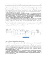
Fig. 24. Estimated magnitudes of the 60 Hz and fifth harmonic for phase A voltage.
The second case represents a continuous dynamic load. The load consists of two six-phase
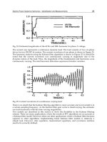
drives for two 200 HP dc motors. The current waveform of one phase is shown in Figure 25.
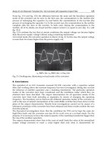
The harmonic analysis using the Kalman filter algorithm is shown in Figure 35. It should be
noted that the current waveform was continuously varying in magnitude due to the
dynamic nature of the load. Thus, the magnitude of the fundamental and harmonics were
continuously varying. The total harmonic distortion experienced similar variation.


Fig. 25. Current waveform of a continuous varying load.
There is no doubt that the Kalman filtering algorithm is more accurate and is not sensitive to
a certain sampling frequency. As the Kalman filter gain vector is time0varying, the estimator
can track harmonics with the time varying magnitudes.
Two models are described in this section to show the flexibility in the Kalman filtering
scheme. There are many applications, where the results of FFT algorithms are as accurate as
a Kalman filter model. However, there are other applications where a Kalman filter becomes
superior to other algorithms. Implementing linear Kalman filter models is relatively a
simple task. However, state equations, measurement equations, and covariance matrices
need to be correctly defined.

Power Quality Harmonics Analysis and Real Measurements Data

30
Kalman filter used in the previous section assumes that the digital samples for the voltage
and current signal waveforms are known in advance, or at least, when it is applied on-line,
good estimates for the signals parameters are assumed with a certain degree of accuracy, so

that the filter converges to the optimal estimates in few samples later. Also, it assumes that
an accurate model is presented for the signals; otherwise inaccurate estimates would be
obtained. Ref. 8 uses the Kalman filter algorithm to obtain the optimal estimate of the power
system harmonic content. The measurements used in this reference are the power system
voltage and line flows at different harmonics obtained from a harmonic load flow program
(HARMFLO). The effect of load variation over a one day cycle on the power system
harmonics and standard are presented. The optimal estimates, in this reference, are the
power system bus voltage magnitudes and phase angles at different harmonic level.


Fig. 35. Magnitude of dominant frequencies and harmonic distortion of waveform shown in
Figure 34 using the Kalman filtering approach.
4.2 Linear dynamic weighted least absolute estimates [11]
This section presents the application of the linear dynamic weighted least absolute value
dynamic filter for power system harmonics identification and measurements. The two
models developed earlier, model 1 and model 2, are used with this filter. As we explained
earlier, this filter can deal easily with the outlier, unusual events, in the voltage or current
waveforms.
Software implementation
A software package has been developed to analyze digitized current and voltage
waveforms. This package has been tested on simulated data sets, as well as on an actual

Electric Power Systems Harmonics - Identification and Measurements

31
recorded data set. and computes the voltage and current harmonics magnitude, the voltage
and current harmonics phase angles, and the fundamental power and harmonics power.
Initialization of the filter
To initialize the recursive process of the proposed filter, with an initial process vector and
covariance matrix P, a simple deterministic procedure uses the static least squares error

estimate of previous measurements. Thus, the initial process vector may be computed as:
1
0
ˆ
TT
XHHHz





and the corresponding covariance error matrix is:
1
0
ˆ
T
PHH







where H is an m  m matrix of measurements, and z is an m  1 vector of previous
measurements, the initial process vector may be selected to be zero, and the first few
milliseconds are considered to be the initialization period.
4.3 Testing the algorithm using simulated data
The proposed algorithm and the two models were tested using a voltage signal waveform of
known harmonic contents described as:











1cos 10 0.1cos 3 20 0.08cos 5 30 0.08cos 9 40
0.06cos 11 50 0.05cos 13 60 0.03cos 19 70
vttttt
ttt
  


  
  


The data window size is two cycles, with sampling frequency of 64 samples/cycle. That is,
the total number of samples used is 128 samples, and the sampling frequency is 3840 Hz.
For this simulated example we have the following results.
Using the two models, the proposed filtering algorithm estimates exactly the harmonic
content of the voltage waveform both magnitudes and phase angles and the two proposed
models produce the same results.
The steady-state gain of the proposed filter is periodic with a period of 1/60 s. This time
variation is due to the time varying nature of the vector states in the measurement equation.
Figure 54 give the proposed filter gain for X

1
and Y
1
.
The gain of the proposed filter reaches the steady-state value in a very short time, since the
initialization of the recursive process, as explained in the preceding section, was sufficiently
accurate.
The effects of frequency drift on the estimate are also considered. We assume small and
large values for the frequency drift: f = -0.10 Hz and f = -1.0 Hz, respectively. In this
study the elements of the matrix H(k) are calculated at 60 Hz, and the voltage signal is
sampled at (

= 2

f, f = 60 + f). Figs. 24 and 29 give the results obtained for these two
frequency deviations for the fundamental and the third harmonic. Fig. 55 gives the
estimated magnitude, and Fig. 29 gives the estimated phase angles. Examination of these
two curves reveals the following:

Power Quality Harmonics Analysis and Real Measurements Data

32

Fig. 27. Gain of the proposed filter for X
1
and Y
1
using models 1 and 2.

Fig. 28. Estimated magnitudes of 60 Hz and third harmonic for frequency drifts using
models 1 and 2.

For a small frequency drift, f = -0.10 Hz, the fundamental magnitude and the third
harmonic magnitude do not change appreciably; whereas for a large frequency drift, f
= -1.0 Hz, they exhibit large relative errors, ranging from 7% for the fundamental to 25%
for the third harmonics.

On the other hand, for the small frequency drift the fundamental phase angle and the
third harmonic phase angle do not change appreciably, whereas for the large frequency

Electric Power Systems Harmonics - Identification and Measurements

33
drift both phase angles have large changes and the estimates produced are of bad
quality.



Fig. 29. Estimated phase angles for frequency drifts using models 1 and 2
To overcome this drawback, it has been found through extensive runs that if the elements of
the matrix H(k) are calculated at the same frequency of the voltage signal waveform, good
estimates are produced and the frequency drift has in this case no effect. Indeed, to perform
this modification the proposed algorithm needs a frequency-measurement algorithm before
the estimation process is begun.
It has been found, through extensive runs that the filter gains for the fundamental voltage
components, as a case study, do not change with the frequency drifts. Indeed, that is true
since the filter gain K(k) does not depend on the measurements (eqn. 8).
As the state transition matrix for model 2 is a full matrix, it requires more computation than
model 1 to update the state vector. Therefore in the rest of this study, only model 1 is used.

4.4 Testing on actual recorded data
The proposed algorithm is implemented to identify and measure the harmonics content for
a practical system of operation. The system under study consists of a variable-frequency
drive that controls a 3000 HP, 23 kV induction motor connected to an oil pipeline
compressor. The waveforms of the three phase currents are given in Fig. 31. It has been
found for this system that the waveforms of the phase voltages are nearly pure sinusoidal
waveforms. A careful examination of the current waveforms revealed that the waveforms
consist of: harmonics of 60 Hz, decaying period high-frequency transients, and harmonics
of less than 60 Hz (sub-harmonics). The waveform was originally sampled at a 118 ms time

Power Quality Harmonics Analysis and Real Measurements Data

34
interval and a sampling frequency of 8.5 kHz. A computer program was written to change
this sampling rate in the analysis.
Figs. 31 and 32 show the recursive estimation of the magnitude of the fundamental, second,
third and fourth harmonics for the voltage of phase A. Examination of these curves reveals
that the highest-energy harmonic is the fundamental, 60 Hz, and the magnitude of the
second, third and fourth harmonics are very small. However, Fig. 33 shows the recursive
estimation of the fundamental, and Fig. 34 shows the recursive estimation of the second,
fourth and sixth harmonics for the current of phase A at different data window sizes.
Indeed, we can note that the magnitudes of the harmonics are time-varying since their
magnitudes change from one data window to another, and the highest energy harmonics
are the fourth and sixth. On the other hand, Fig. 35 shows the estimate of the phase angles of
the second, fourth and sixth harmonics, at different data window sizes. It can be noted from
this figure that the phase angles are also time0varing because their magnitudes vary from
one data window to another.

Fig. 30. Actual recorded current waveform of phases A, B and C.

Electric Power Systems Harmonics - Identification and Measurements

35


Fig. 31. Estimated fundamental voltage.





Fig. 32. Estimated voltage harmonics for V

Power Quality Harmonics Analysis and Real Measurements Data

36


Fig. 33. Estimated fundamental current I
A
.

Fig. 34. Harmonics magnitude of I
A
against time steps at various window sizes.
Furthermore, Figs. 36 – 38 show the recursive estimation of the fundamental, fourth and the
sixth harmonics power, respectively, for the system under study (the factor 2 in these figures
is due to the fact that the maximum values for the voltage and current are used to calculate
this power). Examination of these curves reveals the following results. The fundamental
power and the fourth and sixth harmonics are time-varying.

Electric Power Systems Harmonics - Identification and Measurements

37
For this system the highest-energy harmonic component is the fundamental power, the
power due to the fundamental voltage and current.




Fig. 35. Harmonics phase angles of I
A
against time steps at various window sizes.





Fig. 36. Fundamental powers against time steps.

Power Quality Harmonics Analysis and Real Measurements Data

38

Fig. 37. Fourth harmonic power in the three phases against time steps at various window sizes.
The fundamental powers, in the three phases, are unequal; i.e. the system is unbalanced. The
fourth harmonic of phase C, and later after 1.5 cycles of phase A, are absorbing power from
the supply, whereas those for phase B and the earlier phase A are supplying power to the
network.
The sixth harmonic of phase B is absorbing power from the network, whereas the six
harmonics of phases A and C are supplying power to the network; but the total power is still
the sum of the three-phase power.


Fig. 38. Sixth harmonic powers in the three phases against time steps at various window
sizes.
The fundamental power and the fourth and sixth harmonics power are changing from one
data window to another.

Electric Power Systems Harmonics - Identification and Measurements

39
4.5 Comparison with Kalman Filter (KF) algorithm
The proposed algorithm is compared with KF algorithm. Fig 39 gives the results obtained
when both filters are implemented to estimate the second harmonic components of the
current in phase A, at different data window sizes and when the considered number of
harmonics is 15. Examination of the Figure reveals the following; both filters produce
almost the same estimate for the second harmonic magnitude; and the magnitude of the
estimated harmonic varies from one data window to another.


Fig. 39. Estimated second harmonic magnitude using KF and WLAV.

4.5.1 Effects of outliers
In this Section the effects of outliers (unusual events on the system waveforms) are studied,
and we compare the new proposed filter and the well-known Kalman filtering algorithm. In
the first Subsection we compare the results obtained using the simulated data set of Section
2, and in the second Subsection the actual recorded data set is used.
Simulated data
The simulated data set of Section 4.3 has been used in this Section, where we assume
(randomly) that the data set is contaminated with gross error, we change the sign for some
measurements or we put these measurements equal to zero. Fig. 40 shows the recursive
estimate of the fundamental voltage magnitude using the proposed filter and the well-
known Kalman filtering algorithm. Careful examination of this curve reveals the following
results.
The proposed dynamic filter and the Kalman filter produce an optimal estimate to the
fundamental voltage magnitude, depending on the data considered. In other words, the
voltage waveform magnitude in the presence of outliers is considered as a time-varying
magnitude instead of a constant magnitude.
The proposed filter and the Kalman filter take approximately two cycles to reach the exact
value of the fundamental voltage magnitude. However, if such outliers are corrected, the
discrete least absolute value dynamic filter almost produces the exact value of the
fundamental voltage during the recursive process, and the effects of the outliers are greatly
reduced Figure 41.

Power Quality Harmonics Analysis and Real Measurements Data

40

Fig. 40. Effects of bad data on the estimated fundamental voltage.
Actual recorded data
In this Section the actual recorded data set that is available is tested for outliers’
contamination. Fig. 42 shows the recursive estimate of the fundamental current of phase A

using the proposed filter, as well as Kalman filter algorithms. Indeed, both filters produce
an optimal estimate according to the data available. However, if we compare this figure
with Fig. 42, we can note that both filters produce an estimate different from what it should
be. Fig. 42 shows the recursive estimates using both algorithms when the outliers are
corrected. Indeed, the proposed filter produces an optimal estimate similar to what it should
be, which is given in Fig. 43.


Fig. 41. Estimated fundamental voltage magnitude before and after correction for outliers.

Electric Power Systems Harmonics - Identification and Measurements

41

Fig. 42. Estimated fundamental current when the data set is contaminated with outliers.

Fig. 43. Estimated fundamental current before and after correction for outliers.
4.6 Remarks
 The discrete least absolute dynamic filter (DLAV) can easily handle the parameters of
the harmonics with time-varying magnitudes.

The DLAV and KF produce the same estimates if the measurement set is not
contaminated with bad data.

The DLAV is able to identify and correct bad data, whereas the KF algorithm needs pre-
filtering to identify and eliminate this bad data.
It has been shown that if the waveform is non-stationary, the estimated parameters are
affected by the size of the data window.

Power Quality Harmonics Analysis and Real Measurements Data

42
It has been pointed out in the simulated results that the harmonic filter is sensitive to the
deviations of frequency of the fundamental component. An algorithm to measure the power
system frequency should precede the harmonics filter.
5. Power system sub-harmonics (interharmonics); dynamic case
As we said in the beginning of this chapter, the off-on switching of the power electronics
equipment in power system control may produce damped transients of high and/or low
frequency on the voltage and/or current waveforms. Equation (20) gives the model for such
voltage waveform. The first term in this equation presents the damping inter-harmonics
model, while the second term presents the harmonics that contaminated the voltage
waveform including the fundamental. In this section, we explain the application of the
linear dynamic Kalman filtering algorithm for measuring and identifying these inter-
harmonics. As we said before, the identification process is split into two sub-problems. In
the first problem, the harmonic contents of the waveform are identified. Once the harmonic
contents of the waveform are identified, the reconstructed waveform can be obtained and
the error in the waveform, which is the difference between the actual and the reconstructed
waveform, can be obtained. In the second problem, this error is analyzed to identify the sub-
harmonics.
Finally, the final error is obtained by subtracting the combination of the harmonic and the
sub-harmonic contents, the total reconstructed, from the actual waveform. It has been
shown that by identifying these sub-harmonics, the final error is reduced greatly.
5.1 Modeling of the system sub-harmonics
For Kalman filter application, equation (28) is the measurement equation, and we recall it
here as










Zt Ht t t

 (28)
If the voltage is sampled at a pre-selected rate, its samples would be obtained at equal time
intervals, say t seconds. Then equation (26) can be written at stage k, k = 1, 2, …, k, where K
is the total number of intervals, K = [window size in seconds/t] = [window size in seconds
 sampling frequency (Hz)].















11 1 12 2 16 6
zkt h k tx k h ktx k h ktx k      
 (50)
If there are m samples, equation (8.64) turns out to be a set of equations. Each equation

defines the system at a certain time (kt).









1
zkt Hkt k wk
ii

   ;1,2,,im

 (51)
This equation can be written in vector form as:









zkt Hk t k wk

   (52)

where
z(k) is m  1 measurement vector taken over the window size

Electric Power Systems Harmonics - Identification and Measurements

43

(k) is n  1 state vector to be estimated. It could be harmonic or sub-harmonic
parameters depending on both H(k) and z(k)
H(k) is m  n matrix giving the ideal connection between z(kt) and

(k) in the absence of
noise w(k). If the elements of H(kt) are given by equation (25), it is clear that
H(kt) is a time-varying matrix.
w(k) is an m noise vector to be minimized and is assumed to be random white noise
with known covariance construction.
Equation (52) describes the measurement system equation at time kt.
The state space variable equation for this model may be expressed as 













1
11
1
22
1
33


1
xk xk
xk xk
xk xk
wk
xk xk
uu







(53)
Equation (67) can be rewritten in vector form as:










1kkkwk

  (54)
where

(k) is n  n state transition matrix and it is an identity matrix
w(k) is n  1 plant noise vector
Together equation (52) and (54) form the system dynamic model. It is worthwhile to state
here that in this state space representation the time reference was chosen as a rotating time
reference which caused the state transition matrix to be the identity matrix and the
H matrix
to be a time varying matrix.
Having estimated the parameter vector

, the amplitude, damping constant, and the phase
angle can be determined using equations (30) to (32), at any step
5.2 Testing kalman filter algorithm
5.2.1 Description of the load
The proposed algorithm is tested on an actual recorded data to obtain the damped sub-
harmonics which contaminated the three phase current waveforms of a dynamic load. The
load is a variable frequency drive controlling a 3000 HP induction motor connected to an oil
pipe line compressor. The solid state drive is of 12 pulses designed with harmonic filter. The
data given is the three phase currents at different motor speed, and is given in per unit. The
three phase currents are given in Figure 42. This figure shows high harmonics in each phase
current as well as sub-harmonics. It is clear that the currents have variable magnitudes from
one cycle to another (non-stationary waveforms).
5.2.2 Sub-harmonic estimation

After the harmonic contents of the waveforms had been estimated, the waveform was
reconstructed to get the error in this estimation. Figure 71 gives the real current and the
reconstructed current for phase A as well as the error in this estimation. It has been found

Power Quality Harmonics Analysis and Real Measurements Data

44
that the error has a maximum value of about 10%. The error signal is analyzed again to find
if there are any sub-harmonics in this signal. The Kalman filtering algorithm is used here to
find the amplitude and the phase angle of each sub-harmonic frequency. It was found that
the signal has sub-harmonic frequencies of 15 and 30 Hz. The sub-harmonic amplitudes are
given in
Figure 43 while the phase angle of the 30 Hz component is given in Figure 44. The
sub-harmonic magnitudes were found to be time varying, without any exponential decay, as
seen clearly in Figure 43.


Fig. 42. Actual and reconstructed current for phase
A


Fig. 43. The sub-harmonic amplitudes.

Electric Power Systems Harmonics - Identification and Measurements

45


Fig. 44. The phase angle of the 30 Hz component.
Once the sub-harmonic parameters are estimated, the total reconstructed current can be

obtained by adding the harmonic contents to the sub-harmonic contents. Figure 45 gives the
total resultant error which now is very small, less than 3%.


Fig. 45. the final error in the estimate using KF algorithm.

Power Quality Harmonics Analysis and Real Measurements Data

46
5.2.3 Remarks
 Kalman filter algorithm is implemented, in this section, for identification of sub-
harmonics parameters that contaminated the power system signals.
 By identifying the harmonics and sub-harmonics of the signal under investigation, the
total error in the reconstructed waveform is reduced greatly.
5.3 SUb-harmonics indentification with DLAV algorithm (Soliman and Christensen
algorithm)
In this section, the application of discrete dynamic least absolute value algorithm for
identification and measurement of sub-harmonics is discussed. The model used with
Kalman filter algorithm and explained earlier, will be used in this section, a comparison
with Kalman filter is offered at the end of this section. No needs to report here, the dynamic
equations for the DLAV filter, since they are already given in the previous chapters, in the
place, where we need them. The steps used with Kalman filter in the previous section, will
be followed here. Hence, we discuss the testing of the algorithm.
As we said earlier, the algorithm first estimates the harmonics that contaminated one of the
phases current waveforms, say phase
A; in this estimation, we assumed a large number of
harmonics. The reconstructed waveform and the error for this estimation, which is the
difference between the actual recorded data and the reconstructed waveform, are then
obtained. Figure 46 gives the real current and the reconstructed current for phase
A, as well

as the resultant error. The maximum error in this estimation was found to be about 13%.
This error signal is then analyzed to identify the sub-harmonic parameters. Figure 47 gives
the sub-harmonic amplitudes for sub-harmonic frequencies for 15 and 30 Hz, while Fig. 48
gives the phase angle estimate for the 30 Hz sub-harmonic. Note that in the sub-harmonic
estimation process we assume that the frequencies of these sub-harmonics are known in
advance, and hence the matrix
H can easily be formulated in an off-line mode.


Fig. 46. Actual (full curve) and reconstructed (dotted curve) current for phase
A using the
WLAVF algorithm.

Electric Power Systems Harmonics - Identification and Measurements

47


Fig. 47. Sub-harmonic amplitudes using the WLAF algorithm.



Fig. 48. Phase angle of the 30 Hz component using the WLAVF algorithm.

Power Quality Harmonics Analysis and Real Measurements Data

48

Fig. 49. Final error in the estimate using the WLAVF algorithm.
Finally, the total error is found by subtracting the combination of the harmonic and sub-

harmonic contents, the total reconstructed waveform, from the actual waveform. This error
is given in Fig. 49. It is clear from this Figure that the final error is very small, with a
maximum value of about 3%.
5.4 Comparison between DLAV and KF algorithm
The proposed WLAVF algorithm was compared with the well-known linear KF algorithm.
It can be shown that if there is no gross error contaminating the data, both filters produce
very close results. However, some points may be mentioned here.

Fig. 50. Comparison between the filter gains for component
x
1
.