Anatomy of a Robot Part 13 pps
Bạn đang xem bản rút gọn của tài liệu. Xem và tải ngay bản đầy đủ của tài liệu tại đây (292.29 KB, 20 trang )
Physical Layer
All that said, digital communication comes down to one thing: sending data over a chan-
nel. Another fundamental theorem came out of Shannon’s work (first mentioned in
Chapter 8). It comes down to an equation that is the fundamental, limiting case for the
transmission of data through a channel:
C is the capacity of the channel in bits per second, B is the bandwidth of the channel
in cycles per second, and S/N is the signal-to-noise ratio in the channel.
Intuitively, this says that if the S/N ratio is 1 (the signal is the same size as the noise),
we can put almost 1 bit per sine wave through the channel. This is just about baseband
signaling, which we’ll discuss shortly. If the channel has low enough noise and supports
an S/N ratio of about 3, then we can put almost 2 bits per sine wave through the channel.
The truth is, Shannon’s capacity limit has been difficult for engineers to even
approach. Until lately, much of the available bandwidth in communication channels has
been wasted. It is only in the last couple of years that engineers have come up with
methods of packing data into sine waves tight enough to approach Shannon’s limit.
Shannon’s Capacity Theorem plots out to the curve in Figure 9-1.
There is a S/N limit below which there canot be error free transmission. C is the
capacity of the channel in bits per second, B is the bandwidth of the channel in cycles
C ϭ B ϫ log
2
11 ϩ S>N2
226 CHAPTER NINE
FIGURE 9-1 Shannon’s capacity limit
-
8
0
2
44
66
-2-101234567891011121314151617181920
2
Bits per Hertz
Eb/No
09_200256_CH09/Bergren 4/17/03 11:24 AM Page 226
per second, S is the average signal power, N is the average noise power, No is the noise
power density in the channel, and Eb is the energy per bit. Here’s how we determine the
S/N limit:
Since
Raising to the power of 2,
If we make the substitution of the variable x ϭ Eb ϫ C/No ϫ B, we can use a math-
ematical identity. The limit (as x goes to 0) of (x ϩ 1)
1/x
ϭ e.
We want the lower limit of capacity as the S/N goes down. In the limit, x goes to zero
as this happens. We have to transform the last equation and take the limit as x goes
to zero.
In dB, this number is -1.59 dB. Basically, if the signal is below the noise by a small
margin, we are toast! Figure 9-1 shows this limit on the leftside.
limit Eb>No ϭ .69
limit No>Eb ϭ log
2
e ϭ 1.44
log
2
1x ϩ 12
1>x
ϭ No>Eb
x ϫ log
2
1x ϩ 12
1>x
ϭ C>B
log
2
1x ϩ 12 ϭ C>B
1 ϩ Eb ϫ C>No ϫ B ϭ 2
C>B
Eb ϫ C>No ϫ B ϭ 2
C>B
Ϫ 1
Eb ϫ C>No ϫ B ϭ 2
C>B
Ϫ 1
Eb>No ϭ 1B>C2 ϫ 12
C>B
Ϫ 12
2
C>B
ϭ 1 ϩ 1Eb ϫ C2> 1 No ϫ B2
C>B ϭ log
2
11 ϩ 1Eb ϫ C2> 1No ϫ B22
S ϭ Eb ϫ C
C>B ϭ log
2
11 ϩ S>1No ϫ B22
C ϭ B ϫ log
2
11 ϩ S>N2
N ϭ No ϫ B
S>C ϭ Eb
COMMUNICATIONS 227
09_200256_CH09/Bergren 4/17/03 11:24 AM Page 227
This sets the theoretical limit that any modulation system cannot go beyond. It has
been the target for system designers since it was discovered. The limit will show up
below in the error rate curves of various modulation schemes.
Many ways exist for jamming electrons down wires or waves across the airways. In
all these cases, the channel has a bandwidth. Sometimes the bandwidth is limited by
physics; sometimes the Federal Communications Commission (FCC) limits it. In both
cases, Shannon’s Capacity Theorem applies: putting God and the FCC on equal math-
ematical footing.
A quick aside about the FCC: After college, we constructed and ran a pirate radio sta-
tion out of a private house. We broadcast as WRFI for about two years, playing the music
we felt like playing and rebroadcasting the BBC as our newscast. I was a DJ and a periph-
eral player. We had fake airwave names to hide our identities; mine was Judge Crater.
Finally, after a great run, the FCC showed up at our door to shut us down. They had
tracked us down in a specially modified station wagon with a directional antenna molded
into the roof. They only had to follow a big dashboard display arrow to our door. It turns
out the DJ at the time was playing a Chicago blues album. The FCC agents confessed
that they liked the music so much that they pulled over until the album was complete
before they knocked on the door. The DJ opened the door, the FCC employee folded open
his wallet just like Jack Webb on Dragnet, and the DJ got a look at the laminated FCC
business card. Both sides, in turn, dissolved in laughter. Two hours, and some refresh-
ments later, they departed with our crystal, a very civilized conflict. But I digress.
Here are a couple of web sites and a PDF on Shannon’s Capacity Theorem:
■ www.owlnet.rice.edu/ϳengi202/capacity.html
■ www.cs.ncl.ac.uk/old/modules/1996-97/csc210/shannon.html
■ www.elec.mq.edu.au/ϳcl/files_pdf/elec321/lect_capacity.pdf
Every method of sending data across a channel has a mathematical footing. Often,
the method itself leads to a closed mathematical form for the capacity of the method.
Once the method is implemented, then the implementation can be tested using
Shannon’s Capacity Theorem. Calibrated levels of noise can be added to a perfect chan-
nel and the data-carrying capability can be measured. The testing methods are very
complex and are shown at www.elec.mq.edu.au/ϳcl/files_pdf/elec321/lab_ber.pdf.
Baseband Transmission
Given a wire, it’s entirely possible to turn the voltage off and on to form pulses on the
wire. In its crudest form, this is baseband transmission, a method of communication
distinct from modulated transmission, which we’ll discuss later.
228 CHAPTER NINE
09_200256_CH09/Bergren 4/17/03 11:24 AM Page 228
Baseband transmission is used with many different types of media. Data transmis-
sion by wire has occurred since well before Napoleon’s army used the fax machine.
Yes, the first faxes dropped on the office floor about that time in history (www
.ideafinder.com/history/inventions/story051.htm).
Baseband transmission is also used in tape drives and disks. Data is recorded as
pulses on tape and is read back at a later time.
A sequence of pulses can be constructed in many different ways. Engineers have nat-
urally come up with dozens of different ways these pulses can be interpreted. As is often
the case, other goals exist besides just sending as many bits per second across the chan-
nel as possible. However, in satisfying other goals, channel capacity is sacrificed. Here’s
a list of other goals engineers often have to solve while designing the way pulses are
put into a channel:
■ Direct Current (DC) balance Sometimes the channel cannot transmit a DC
voltage at all. A continuous string of all ones might simply look like a continu-
ously high voltage. Take, for instance, a tape drive. The basic equation for voltage
and the inductance of the tape head coil is
V is the input signal, L is the inductance of the tape head’s coil, and I is the current
through the coil. If V were constant, we’d need an ever-increasing current through
the coil to make the equations work. Since this is impossible, tape designers need
an alternate scheme. They have come up with a coding of the pulses such that an
equal number of zeroes and ones feed into the tape head coil. In this way, the DC
balance is maintained. Only half as many bits can be written as before, but things
work out well. The codes they use are a version of nonreturn to zero (NRZ).
■ Coding for cheap decoders Some data is encoded in such a way that the
decoder can be very inexpensive. Consider, for the moment, pulse-width-encoded
analog signals. A pulse is sent every clock period, and the duty cycle of the pulse
is proportional to a specific analog voltage. The higher the voltage, the larger the
duty cycle, and the bigger percentage of time the pulse spends at a high voltage.
At the receiver, the analog voltage can be recovered using just a low-pass filter
consisting of a resistor and a capacitor. It filters out the AC values in the wave-
form and retains the DC. These types of cheap receiver codes are best used in sit-
uations where there have to be many inexpensive receivers.
■ Self-clocking Some transmission situations require the clock to be recovered at
the receiving end. If that’s the case, select a pulse-coding scheme that has the clock
built into the waveform.
■ Data density Some pulse-coding schemes pack more bits into the transmission
channel than others.
V ϭ L ϫ dI>dt
COMMUNICATIONS 229
09_200256_CH09/Bergren 4/17/03 11:24 AM Page 229
■ Robustness Some pulse-coding schemes have built-in mechanisms for avoid-
ing and/or detecting errors.
The following PDFs and web site provide a good summary of the advantages and dis-
advantages of various coding methods:
■ www.elec.mq.edu.au/ϳcl/files_pdf/elec321/lect_lc.pdf
■ />■ www.cise.ufl.edu/ϳnemo/cen4500/coding.html
PULSE DISTORTION: MATCHING FILTERS
One of the difficult problems with the transmission of pulses through a channel (wire,
fiber optics, or free space) is that the pulses become distorted. What actually happens
is that the pulses spread out in time. If the overall transmission channel has sharp fre-
quency cutoffs, as is appropriate for a densely packed channel, then the pulses come out
of the receiver looking like the sinc function we looked at earlier. The pulse has spread
out over time (see Figure 9-2).
If we try to pack pulses like this tightly together in time, they will tend to interfere
with each other. This is commonly called Intersymbol Interference (ISI), which we will
discuss later (see Figure 9-3).
But there’s a kicker here. A transmission channel cannot be perfect, with sharp
rolloffs in frequency. As a practical matter, we must allow extra bandwidth and relax
our requirements on the transmission channel and the transmission equipment. A com-
mon solution to this problem is the Raised Cosine Filter (RCF), a filter we saw before
in Chapter 8 as the Hanning window. A common practice is to include this matching
RCF in the transmitter to precompensate the pulses for the effect of the channel. The
230 CHAPTER NINE
FIGURE 9-2 Received pulses spread out to look like the sinc function.
-0.4
-0.2
0
0.2
0.4
0.6
0.8
1
1.2
1
SINC (t/T)
time t
T0
2T
Amplitude
09_200256_CH09/Bergren 4/17/03 11:24 AM Page 230
received pulse signals, even though they have oscillations in their leading and trailing
edge, cross zero just when the samples are taken. That way, adjacent pulses do not inter-
fere with one another (see Figure 9-4).
The following sites discuss the RCF:
■ www.iowegian.com/rcfilt.htm
■ www-users.cs.york.ac.uk/ϳfisher/mkfilter/racos.html
■ www.ittc.ukans.edu/ϳrvc/documents/rcdes.pdf
■ www.nuhertz.com/filter/raised.html
COMMON BASEBAND COMMUNICATION STANDARDS
The following are some relatively common wired baseband communication links that
we all have used. These are communication links that have relatively few wires and are
COMMUNICATIONS 231
FIGURE 9-3 A poor receive filter enables consecutive pulses to interfere
with each other.
Intersymbol Interference
FIGURE 9-4 A good raised cosine receive filter makes consecutive pulses
cooperate.
All pulses cross 0 at decision time.
09_200256_CH09/Bergren 4/17/03 11:24 AM Page 231
generally considered serial links. Many computer boards come already wired with these
sorts of communication ports, and many interface chips are available that support them.
■ RS232/423 RS232/423 has been around since 1962 and is capable of sending
data at up to 100 Kbps (RS423) over a three-wire interface. It is considered to be
a local interface for point-to-point communication. It’s supposed to be simple to
use, but it can cause a considerable amount of grief because many optional wires
and different pinouts exist for various types of connectors. Other than the physi-
cal layer and the definition of bit ordering, very little layering takes place above
the physical layer with RS232. For more info, go to www.arcelect.com/rs232.htm
and www.camiresearch.com/Data_Com_Basics/RS232_standard.html.
■ RS422 RS422 uses differential, balanced signals, which are more immune from
noise than RS232’s single-sided wiring. Data rates are up to 10 Mbps at over 4,000
feet of wiring. Other than the physical layer and the definition of bit ordering, very
little layering is done with RS422 (also see www.arcelect.com/rs422.htm).
■ 10BT/100BT/1000BT networking Ethernet is one of the most popular local
area network (LAN) technologies. 10BT LAN technology enables most business
offices to connect all the computers to the network. The computers can transmit
data to one another at speeds approaching 9 to 10 million bits per second. As a
practical matter, on busy networks, the best rates a user can achieve are much
lower. The software stack includes up to four layers from physical layer 1 (network
interface [NIC] cards), up to IP, and to TCP at layer 4.
100BT is 10 times faster than 10BT. 1000BT is 10 times faster again and avail-
able for use with a fiber-optic physical layer as well as copper wiring. See these
web sites and PDF files for more info:
■ www.lantronix.com/learning/tutorials/
■ www.lothlorien.net/collections/computer/ethernet.html
■ />■ www.10gea.org/GEA1000BASET1197_rev-wp.pdf
Modulated Communications
Sometimes digital communications just cannot be sent over a channel without modula-
tion; baseband communications will not work. This might be the case for several reasons:
■ Sometimes wiring is not a possibility because of distance. Unmodulated data sig-
nals are generally relatively low in frequency. Transmitting a slower baseband sig-
nal through an antenna requires an antenna roughly the size of the wavelength of
232 CHAPTER NINE
09_200256_CH09/Bergren 4/17/03 11:24 AM Page 232
the signal itself. For an RS232 signal at 100 Kbps, the signal has a waveform with
about 10 microseconds per bit. Light travels 3,000 meters, about 2 miles, in 10
microseconds. We’d need an antenna two miles long to transmit such a signal effi-
ciently into the impedance of space. Clearly, this won’t work well. It’s one of the
primary reasons almost no baseband wireless communication systems exist. They
almost all use modulation.
■ Sometimes the channel is so noisy that special techniques must be used to encode
the signal prior to transmission.
■ The FCC and other organizations regulate the use of transmission spectra.
Communication links must be sandwiched between other communication links in
the legal communication bands. To keep these competing communication links
separate, precision modulation is used.
Modulation generally involves the use of a carrier signal. The information signal (I)
is mixed (multiplied by) the carrier signal (C), and the modulated signal (M) is broad-
cast through the communication channel:
Although many different signals can be used as the carrier C, the type of signal most
often used is the sine wave. Although the operation x can be just about any type of oper-
ation, the most common type of mixing involves multiplication.
A sine wave only has a few parameters in its equation. Thus, modulating a carrier
sine wave can only involve a few different operations:
where A is the amplitude, v is the frequency, and u is the phase.
Any modulation of this carrier wave by the data must involve a modification of one
or more of these three parameters. One or more of the parameters (A, v, or u) may take
on one or more values based on the data. As the data input, I, takes on one of n differ-
ent values, the modulated carrier wave takes on one of n different shapes to represent
the data I. The following 3 discussions describe modulating A, v, and u in that order.
■ Amplitude Shift Keying (ASK) sets
where A is one of n different amplitudes, v is the fixed frequency, and u is the
fixed phase. In the simplest form, n ϭ 2, and the waveform M looks like a sine
wave that vanishes to zero whenever the data is zero (A ϭ 0 or 1).
M1n2 ϭ An ϫ sin 1v ϫ t ϩ u 2
C ϭ A ϫ sin 1v ϫ t ϩ u2
M ϭ I ϫ C
COMMUNICATIONS 233
09_200256_CH09/Bergren 4/17/03 11:24 AM Page 233
■ Frequency Shift Keying (FSK) sets
where A is the fixed amplitude, vn is one of n different frequencies, and u is the
fixed phase. In the simplest form, n ϭ 2, and the waveform M looks like a sine
wave that slows down in frequency whenever the data is zero (v ϭ freq0 or freq1).
■ Phase Shift Keying (PSK) sets
where A is the fixed amplitude, v is the fixed frequency, and un is one of n dif-
ferent phases. In the simplest form, n equals 2, and the waveform M looks like a
sine wave that inverts vertically whenever the data is zero (u ϭ 0 or 180 degrees).
Each modulation method has a corresponding demodulation method. Each modula-
tion method also has a mathematical structure that shows the probability of making
errors given a specific S/N ratio. We won’t go into the math here since it involves both
calculus and probability functions with Gaussian distributions. For further reading on
this, please see the following web site and PDF file:
■ www.sss-mag.com/ebn0.html
■ www.elec.mq.edu.au/ϳcl/files_pdf/elec321/lect_ber.pdf
What comes out of the calculations are called Eb/No curves (pronounced “ebb no”).
They look like the following figure, which shows a bit error rate (BER) versus an
Eb/No curve for a specific modulation scheme (see Figure 9-5).
Remember, Eb/No is the ratio of the energy in a single bit to the energy density of
the noise. A few observations about this graph:
■ The better the S/N ratio (the higher the Eb/No), the lower the error rate (BER). It
stands to reason that a better signal will work more effectively in the channel.
■ The Shannon limit is shown as a box. The top of the box is formed at a BER of
0.50. Even a monkey can get a data bit right half the time! The vertical edge of the
box is at an Eb/No of 0.69, the lower limit of the digital transmission we derived
earlier. No meaningful transmission can take place with an Eb/No that low; the
channel capacity falls to zero.
■ This graph shows the BER we can expect in the face of various Eb/No values in
the channel. Adjustments can be made. If the channel has a fixed No value that
cannot be altered, an engineer can only try to increase Eb, perhaps by increasing
the signal power pumped into the channel.
M1n2 ϭ A ϫ sin 1v ϫ t ϩ un2
M1n2 ϭ A ϫ sin 1vn ϫ t ϩ u2
234 CHAPTER NINE
09_200256_CH09/Bergren 4/17/03 11:24 AM Page 234
■ Conversely, if an engineer needs a specific BER (or lower) to make a system work,
this specifies the minimum Eb/No the channel must have. In practice, a perfect
realization of the theoretical Eb/No curve cannot be realized and an engineer
should condition the channel to an Eb/No higher than that theoretically required.
Figure 9-6 shows two BER curves from two different but similar modulation
schemes. These curves show that some modulation schemes are more efficient than oth-
ers. In fact, the entire game of building modulation schemes is an effort to try to
COMMUNICATIONS 235
FIGURE 9-5 S/N effect: As the power per bit (Eb/No) goes up, the bit error
rate (BER) goes down.
-6
-5
-4
-3
-2
-1
0
-10 -5 0 5 10 15 20 25
Eb/No (dB)
Log (BER)
Shannon's
Limit
-1.6 dB
FIGURE 9-6 A better modulator (the inner curve) can approach the Shannon
limit more closely.
-6
-5
-4
-3
-2
-1
0
-10 -5 0 5 10 15 20 25
Eb/No (dB)
Log (BER)
Shannon's
Limit
-1.6 dB
09_200256_CH09/Bergren 4/17/03 11:24 AM Page 235
approach the Shannon limit. As might be expected, more efficient modulators are more
expensive. Most people settle for wasting bandwidth rather than paying for a more
expensive modulator.
COMPLICATED MODULATORS
These previous examples are very rudimentary modulation schemes. Often, in modern
modulation methods, more than one carrier parameter is modulated at the same time.
Let’s also introduce here the concept of a symbol. A symbol is simply a multiple bit
number used for modulation. A byte could be an 8-bit symbol used in ASK to set the
amplitude to one of 256 different levels. The process of modulating the carrier by a sym-
bol changes the character of the carrier waveforms.
The receiver demodulates the data and makes an attempt to determine the character
of the waveform in order to classify which symbol it represents. The demodulator in the
receiver serves to quantify the received waveform into a symbol space. Visualize the
symbol space as a multidimensional data space within which the received signal is mov-
ing. As the amplitude, frequency, and phase of the received signal change, the signal
moves around in the receiver’s symbol space. If, for instance, 256 different symbols are
defined, then 256 different points are in the symbol space where these symbols reside.
If the received signal is crossing one of these 256 points when the data clock ticks, the
received symbol associated with that point is chosen as the received symbol, and the
data (8 bits) represented by that symbol is dumped into the receiver’s output.
Let’s look at a simplified example. Suppose we are modulating both amplitude and
phase with one bit each. Four different symbols (00, 01, 10, and 11) would be used and
the symbol space might look like Figure 9-7.
236 CHAPTER NINE
FIGURE 9-7 A graph of a simple symbol space
X
X
X
X
1100
10
01
09_200256_CH09/Bergren 4/17/03 11:24 AM Page 236
When the data clock ticks, we sample the position of the received signal in symbol
space. Suppose we receive a symbol whose amplitude is a little low but has a very clear
phase. It might map into the following point shown in Figure 9-8.
To decide on which symbol is received, we put a decision grid into symbol space, as
shown in Figure 9-9. The decision grid makes the decision quickly, and the symbol is
resolved to be 01.
It’s clear that we do not want symbols to be too close together in symbol space.
Modulation schemes are designed to minimize the probability that symbols will be too
close or that the peculiarities of the channel will cause one symbol to be mistaken for
another.
COMMUNICATIONS 237
FIGURE 9-8 Classifying a recently received symbol that is shown as “?”
X
X
X
X
1100
10
01
?
FIGURE 9-9 A hard decision grid classifies the received symbol as 01.
X
X
X
X
1100
10
01
?
Decision
Grid
? = "01"
09_200256_CH09/Bergren 4/17/03 11:24 AM Page 237
A more complex example of this sort of symbol space is 64 Quadrature Amplitude
Modulation (QAM), where 8 bits of data are modulated at the same time. Symbol space
for 64 QAM might have a square structure as shown in Figure 9-10.
The incoming symbol data traces a wild pattern through the 8 ϫ 8 grid of dots. To a
certain extent, because the symbol data tries to stick to the grid points, the grid has open
areas where the data does not traverse. These open areas look like eyes and are the sub-
ject of the next discussion.
Error Control
Designers of big symbol spaces have to worry about what’s called the open eye.
Remember, when the data clock ticks in the receiver, the received signal should be right
on top of a symbol point. To get there from any other symbol point, it should travel
along a well-known route through symbol space (governed by the shape of the carrier
signal). With a noiseless channel, the trail of the received signal would trace a very nice
set of geometric paths and lots of empty space would be showing on the symbol space,
places where the signal never traverses. These empty spaces are what engineers look for
when they are trying to find the open eye. These spaces are called that because they are
generally formed by two sine waves and have the shape shown in Figure 9-11.
A good engineer can put the communication waveform on an oscilloscope (or other
instrument), look at the eye pattern, and determine the health of the physical layer of
the communication network.
238 CHAPTER NINE
FIGURE 9-10 A symbol space for 64 QAM
x x x x x x x x
x x x x x x x x
x x x x x x x x
x x x x x x x x
x x x x x x x x
x x x x x x x x
x x x x x x x x
x x x x x x x x
09_200256_CH09/Bergren 4/17/03 11:24 AM Page 238
In the same manner, engineers can plot the recent data points to see how tightly they
cluster around the symbol points. A healthy communication link will have a very tight
clustering around the symbol points, and a sickly system will have them spread out in
a sloppy manner.
These are all ways to try to keep the physical link healthy, but steps can be taken in
the design of the communication link that will make it more robust. Many different
ways are available for looking at what these techniques represent. I prefer to think of
them all the same way: sending the data more than once.
In a situation where noise might ruin data inside the channel, the receiver is more
likely to get the data if it’s sent more than once. If the receiver is smart enough to rec-
ognize when data is corrupt, it can just wait for the second helping of the same data.
This becomes particularly important for robots in remote locations.
Sending duplicate data can be done in many different ways. Clearly, it’s possible to
just send the data twice or three times. But believe it or not, it’s possible to send the data
1.5 times, 1.1 times, or even 1.01 times.
Within certain bounds, robot designers can choose among communication protocol
codes that enable them to pick the amount of redundancy built into the communication
link. Since redundant data consumes bandwidth, this allows the designers to decide how
much of the bandwidth is wasted. Sending extra data effectively lowers the BER, since
errors are corrected at the receiver. Getting a lower BER is almost the equivalent of hav-
ing a better Eb/No. Thus, designers can say they get coding gain out of different com-
munication protocol codes. This coding gain can actually be realized since the coding
gain can be subtracted off the Eb/No in the actual channel to get the same BER in a
given situation. Add coding gain, decrease the Eb/No gain, and come out even. In prac-
tice, however, most engineers take the coding gain on top of the existing Eb/No and
realize their profit as a lower BER.
COMMUNICATIONS 239
FIGURE 9-11 An open-eye diagram showing received signal traces crossing
two symbol space X’s
X X
Symbol 'X' is under each crossing
09_200256_CH09/Bergren 4/17/03 11:24 AM Page 239
This happens in satellite communications all the time. In fact, most satellite com-
munication links are designed and specified with the coding gain built right into the
communication protocol. Since many of the codes have parametric options, it is possi-
ble for the operator of a satcom link to pick a code on the fly that matches the quality
of the channel. If the satcom link has a low No, then little coding gain may be needed
and the data rate can go up. If the satellite link has a high No, then a stronger coding
gain may be needed to maintain the quality of the data at the expense of a lower
data rate.
ERROR DISTRIBUTION
Robot designers must also take a very careful look at the channel. It’s one thing to pre-
dict the BER from the modulation method and coding, but it does no good at all if
sunspots wreck the transmission for minutes or seconds at a time. Error rates are con-
catenated; all the links in the communication chain must be functioning at the same
time. An error in any one link may, or may not, be corrected in another link down the
chain.
In addition, noise is unpredictable. That’s why they call it noise in the first place.
Granted, it has certain mathematical properties that are dependable in the average, but
random events can lead to a burst of errors that may not be caught by the coding scheme
chosen. We must look at the density and distribution of errors in the channel, in addi-
tion to the error rate.
One thing further must be said about the distribution of errors. Some coding schemes
(like Viterbi, which we’ll get to soon) gather up errors all together in a net and correct
them all at once. The problem is, if something goes wrong and they cannot all be cor-
rected, the net rips and a local flood of errors happens that would not have occurred nat-
urally in such a manner. This type of situation is actually caused by the error-correction
coding scheme. The system must be prepared to survive such an event. We’ve probably
all seen such error bursts in the middle of soccer games from overseas. The game goes
along fine until there’s a massive burst of black and green blocks on the screen. We’ll
see why this occurs shortly.
Let’s take a look at some of the coding methods that send duplicate data. The differ-
ent techniques have the same basic purpose: to decrease the error rate by sending some
of the data more than once. The techniques are basically divided into two different meth-
ods. Some communication channels are bidirectional, and many are not. A bidirectional
communication channel enables the retransmission of data by request of the receiver; a
unidirectional communication channel does not.
240 CHAPTER NINE
09_200256_CH09/Bergren 4/17/03 11:24 AM Page 240
BIDIRECTIONAL COMMUNICATION CHANNELS
A bidirectional communication channel enables the receiver to send the transmitter
information about the state of the channel and the integrity of the received data.
Several tools are used in a bidirectional communication channel to help send duplicate
data. These tools are not confined to use in a bidirectional channel, but they can be used
to take maximum advantage of the reverse communications link. In fact, all the tools
used in a unidirectional communication channel will also work in a bidirectional
channel.
BLOCK CHECKSUMS
When the receiver receives data, it must determine, to the extent possible, whether the
channel has changed the data. It does not matter where in the channel the data was
changed. Noise from lightening storms or sunspots may have changed the data en route
or the receiver might have had a temporary power glitch. The only thing that counts is
whether the receiver’s data buffer got the same data that was transmitted. Much like
aspirin bottles that come with a safety seal that ensures protection, data can be wrapped
in a checksum that will guarantee the integrity of the data.
A checksum is a series of data bits that serve to summarize a block of data. The
sender can chop the data stream into a series of blocks that may be many bytes long.
The checksum is computed and appended to the data block before transmission. We’ll
discuss just how checksums are computed later. The receiver knows, by prior arrange-
ment, how the checksum will be computed. The receiver, upon receiving the data block
(and checksum), independently computes the checksum again and compares it to the
received checksum. If the results are different, then a problem exists. If the checksums
are the same, then the data is accepted and the receiver moves on to the next block. But
suppose a problem exists. In this case, several different actions are possible.
Single Error Detection
If the transmitted checksum information has relatively few bytes, it’s possible that an
error can only be detected. There may not be enough information to either correct the
error or to even detect more than one error in the data block. If an error is detected, the
receiver can ask the transmitter to retransmit the block of information. One protocol
used in the retransmission of data is discussed later.
COMMUNICATIONS 241
09_200256_CH09/Bergren 4/17/03 11:24 AM Page 241
Multiple Error Detection
If the checksum has enough data in it (and the appropriate mathematical structure), then
it may be possible to detect more than one error in the data block. Note this means that
a weak checksum method (with little data in the checksum) may even fail to detect any
error if more than one error occurs in the data block.
Consider the nature of the communication channel used in the robot. If it is possible
for more than one error to occur at the same time, then try a checksum method capable
of at least detecting multiple errors. It is certainly possible for multiple errors to occur
at the same time in any communications channel. The key question a robot designer
should examine is the likelihood of such an occurrence. Examine the probability of
errors and the distribution of the errors. Assuming the error rates are small and that the
errors occur independently, it’s safe to assume the chance of two simultaneous errors in
a block is roughly the square of the chance of a single error in a block. The robot
designer should compute this dual error rate and determine if it will be an acceptable
error rate if such errors slip through.
Single Error Correction
If the checksum contains sufficient data to not only detect the existence of an error but
correct it as well, then the data can be corrected before the receiver moves on to the next
block of data. No retransmission from the transmitter will be required. It should be
noted that even error correction schemes will occasionally make mistakes. The strength
of the error-correcting code lies in the mathematics of the protocol. Some errors may
not even be detected, some errors may not be correctable, and some errors will be incor-
rectly corrected. When employing such methods, the robot designer must examine these
error rates and compare them to the allowable error rate.
Multiple Error Correction
Some checksums have sufficient information to correct simultaneous errors. All the
same precautions should be taken as outlined previously. Be aware that such strong
checksums often consume a good deal of bandwidth sending extra checksum data; the
checksums may contain many bytes.
Checksums are smaller blocks of data that summarize larger blocks of data. Often
checksums are called cyclic redundancy checks (CRC). The following web sites will
point out a small difference. Certainly, if a checksum contains more data than the block
it summarizes, then it is not of much use. The whole idea is to summarize the block of
transmitted data in a small number of bytes in an effort to be efficient. Often, a check-
242 CHAPTER NINE
09_200256_CH09/Bergren 4/17/03 11:24 AM Page 242
sum will consist of 1 to 8 bytes of extra information summarizing a block of data that
is between 32 and 1,024 bytes long. These numbers are arbitrary, but common. TCP/IP,
for instance, typically has blocks of data 512 bytes long with checksums that are 2 bytes
long.
Descriptions of the IP checksum method can be found at:
■ www.ietf.org/rfc/rfc1071.txt
■ www.netfor2.com/checksum.html
Here are descriptions of TCP checksums:
■ www.netfor2.com/tcpsum.htm
■ />An interesting statistical analysis of TCP/IP checksum errors in a real-world appli-
cation can be downloaded from www.acm.org/sigcomm/sigcomm2000/conf/paper/sig-
comm2000-9-1.pdf.
The astute observer will note that a data block of 512 bytes can be filled in 2
512ϫ8
dif-
ferent ways. However, a checksum with just 2 bytes can only take on 65,535 (2
2ϫ8
) dif-
ferent checksum values. This means that for each possible checksum value, about 2
256
(or about 7.4 x 10
19)
data blocks will have the very same checksum.
So how do we get away with saying that this sort of checksum is sufficient for an
application? If an error occurs, the erroneous data block just might be identical to one
of the several billion data blocks with the same checksum. The key thing to remember
is that a single error should result in an erroneous data block with only one chance in
65,536 of having the same checksum. If this decrease in the error rate is not good
enough, then design the robot with a stronger checksum, which is perhaps longer.
Certainly, as the mathematical algorithm is chosen for the checksum calculation, make
sure the most common errors all result in a checksum change.
For example, an error in a single bit may be common and should result in a different
checksum. The calculation method for checksums is often described by a polynomial,
a mathematical way to describe the calculations involved in computing a checksum. The
mathematics behind the selection of a good polynomial are beyond the scope of this
book. Fortunately, many standard polynomials (some listed later) exist and we can select
among them without reinventing them.
The following web sites describe using polynomials for the computation of check-
sums:
■ www.4d.com/ACIDOC/CMU/CMU79909.HTM
■ www.geocities.com/SiliconValley/Pines/6639/docs/crc.html
■ www.relisoft.com/Science/CrcMath.html
COMMUNICATIONS 243
09_200256_CH09/Bergren 4/17/03 11:24 AM Page 243
■ www.relisoft.com/Science/CrcNaive.html
■ www.relisoft.com/Science/CrcOptim.html
■ www.relisoft.com/Science/source/Crc.zip
PARITY BITS
Let’s look at a simple checksum structure example. Parity bits, as part of a checksum
structure, can simply indicate how many ones are in a byte. Basically, take a byte and
count up the number of ones in the 8 bits. If we are using an even parity scheme, then
the number of ones in the bits (including the parity bit) must be even. For example, if an
even number of ones is in the data byte, then append a ninth parity bit containing a zero
to the byte to keep an even parity. If the number of ones in the byte is odd, then append
a one as the ninth parity bit to attain even parity. If we do this for every byte in the data
block, then single bit errors in any byte will “finger” that byte as bad. We will be able
to detect single bit errors in the data block at the expense of increasing the data by 1/8.
If we also compute the parity for each bit, over the entire data block we will get more
capability. We can, for example, compute the number of ones in the 0 bit position for
the entire data block and append a column parity byte at the end of the data block con-
taining a single 9-bit number. The column parity byte will contain the parity computed
for the 0th, first, second, . . . eighth, and ninth columns of bits in the data block. Then,
if a single bit is corrupted in the data block, that byte’s parity bit will signal which byte
is erroneous, and the column parity byte will tell us which bit is wrong in that byte. This
will allow us to correct single bit errors in a data block by duplicating and expanding
the data block by about 1/8. It’s not a very strong code; better ones can be created.
It is easy to make up our own code, but we must be sure it matches the requirements
of the robot’s operating environment. The strength of the code should match the error
rates, the error distribution, and the tolerance the robot has for errors.
REED-SOLOMON CHECKSUMS
One of the most often used checksum calculations is the Reed-Solomon (RS) code. This
type of code is capable of correcting multiple errors in a block of data. The reason this
is useful will be outlined shortly. RS coding also expands the data block by appending
parity bytes.
One popular RS code is RS(255,233), which expands a 233-byte data block to 256
bytes by appending 32 bytes of parity checksums, an expansion of the data block by a
factor of about 14 percent. The RS(255,233) polynomial enables up to 16 different bytes
to be corrected at the same time.
244 CHAPTER NINE
09_200256_CH09/Bergren 4/17/03 11:24 AM Page 244
Another popular RS code is used in satellite video transmissions. The Digital Video
Broadcast-Satellite (DVB-S) standard has been standardized on MPEG2 video transmis-
sion using, among other codes, RS(204,188). This code appends 16 parity checksum bytes
to a data block of 188 bytes for a code expansion of about 8.5 percent. The RS(204,188)
polynomial enables up to eight different bytes to be corrected at the same time.
The following web sites and PDF file outline RS encoding and decoding:
■ www.4i2i.com/reed_solomon_codes.htm
■ www.siam.org/siamnews/mtc/mtc193.htm
■ />■ />■ www.elektrobit.co.uk/pdf/reedsolomon.pdf
For fun, go to www.mat.dtu.dk/people/T.Hoeholdt/DVD/index.html, which shows RS
corrections in real time in a very graphic manner. The web page displays an image, shows
graphically the amount of redundant data, enables us to introduce errors in the graphics
image using the mouse, and corrects the errors before our eyes. If too many errors are
introduced, the errors cannot be corrected. This illustrates the limits of block encoding.
RETRANSMISSION
If an error is detected, the receiver can send a NACK, or Negative Acknowledge, back
to the transmitter. This NACK message will request the retransmission of the faulty data
block. Some bidirectional communication protocols call for the receiver to transmit an
acknowledge (ACK) message to acknowledge the reception of every perfectly good data
block. If the communication channel imposes a significant delay on transmissions (such
as what might occur to a remote space probe’s robot), then sending an ACK (or NACK)
message for every data block is impractical. If the transmission protocol enables the
transmitter to transmit multiple blocks of data without receiving messages from the
receiver, then the transmitter must append an identifier to each data block sent.
The identifier is often just a sequential count sufficient to distinguish each data block
from its adjacent neighbors. The receiver, upon identifying a bad checksum, appends
the identifier of the bad block to the NACK message for that block. When the trans-
mitter receives the NACK message, it reassembles the data block that corresponds to
the identifier and retransmits it. The receiver must compute the checksum of the
received retransmission and accept the data block. Note that this will require both the
receiver and the transmitter to buffer (keep) multiple blocks of data in memory during
the transmission cycle.
COMMUNICATIONS 245
09_200256_CH09/Bergren 4/17/03 11:24 AM Page 245