Complex Robotic Systems - Pasquale Chiacchio & Stefano Chiaverini (Eds) Part 5 pptx
Bạn đang xem bản rút gọn của tài liệu. Xem và tải ngay bản đầy đủ của tài liệu tại đây (663.33 KB, 15 trang )
2.4. Illustrative examples
53
0~
0
-o.S
-1
-,.S
-1.S -I
I • I
-0.5 0 0.5 1 1.5 2 2.5 3 3.5
Figure 2.10: Unstable configuration.
unstable configuration means that the mechanism cannot resist x direction
force applied at the task frame.
When the mechanism is near an unstable configuration, it may not be
unstable mathematically, but the ellipsoid will be badly conditioned. As
shown in Figure 2.11, the motion in the x direction is much larger than
in the y direction. When the mechanism moves in to the unstable config-
uration, the ellipsoid becomes infinite in the x direction. From the force
perspective, this suggests that a nearly unstable configuration is also highly
undesirable as large forces from the active joints are needed to counteract
disturbance force at the task frame. We have constructed a physical 3DOF
Stewart Platform, and have indeed verified that unstable and nearly unsta-
ble configurations can have large internal motion with all the active joints
locked. When the ellipsoid is well conditioned, such internal motion is no
longer possible.
2.4.3 Six-DOF Stewart platform example
We now consider a 6-DOF Stewart Platform. Let the three base nodes be
at
[:01] [ ] [0]
Xl
1 x2 = x3 = 1 .
0
54
Chapter 2. Kinematic manipulability of genera/mechanical systems
-0,
-1
-l~'*.s -~ -o,s o o.s '~ 1.s 2 zs 3 3,s
Figure 2.11: Nearly unstable configuration.
The top platform is an isosceles triangle with the two equal sides of length
1.12 and the third side of length 1. The task velocity, VT, is defined as
the translational velocity of the half way point of the line perpendicular to
the base of the isosceles platform• As in the two previous examples, the
task velocity only involves the linear motion but the constraints need to
include orientation. Therefore, the kinematics developed in Section 2.2.1
needs to be slightly modified. With 0 as defined in (2.8), the task velocity
kinematics is now
el -dtelx 03x3 13×3 ]
". " 0 = • VT.
e6 -d6e6x 03x3 I3x3
(2.36)
The constraint equation, (2.1), is the same as in Section 2.2.1, given by
(2.11).
The velocity ellipsoids of the Stewart Platform in three different con-
figurations are shown in Figures 2.12- 2.14 (the force ellipsoids have the
same principal axes but reciprocal length). In the first case, the platform
is horizontal. In the second case, the task frame is rotated 45 ° about the
axis [ 0.71 0.71 0 IT. In the third case, the task frame is rotated 22.5 °
about the vertical axis [ 0 0 1 ].
In each case, three ellipses lying in the plane generated by two of the
principal axes are shown. In the first case, the ellipse is well conditioned
2.5. Effects of
arm
posture and bracing on manipulability
55
2
1.5
1
0.5
N 0
-0.5
-1
-1.5.
-2:
2
0 0 I
y -2 -2 X
Figure 2.12: 3D ellipsoid for 6-DOF Stewart platforms: Case 1.
with the lengths of principal axes: {1.78, 1.43,0.81}. In the second case,
the ellipsoid becomes less well conditioned, the lengths of the principal axes
are {2.31, 1.62, 0.29}. The motion parallel to the platform is more difficult
than other directions. In the third case, the lengths of the principal axes are
{5.62, 1.69, 1.49}. Even though the ellipsoid is fairly welt conditioned (con-
dition number of the singular values is 3.78), but external forces along the
principal axis that corresponds to 5.62, [ -0.54 0.12 -0.83 ], cannot
be resisted as easily as in other directions.
2.5
Effects of arm posture and bracing on
manipulability
In this section, we consider the effect of arm posture, bracing, and grasp
type on the manipulability of the arm (and therefore the ellipsoid).
2.5.1 Effect of arm
posture
For nonredundant arms, there is little choice in positioning the robot joints
in order to allow the end-effector to perform some task. For redundant
arms, there is much more flexibility, allowing the joints to be positioned in
a way which makes it easier for the arm to perform the desired task.
56
Chapter 2. Kinematic manipulability
of
genera/mechanical
systems
2
1
0,8
N 0
-0.5
-1
-1.5
0 0
y -2 -2
X
Figure 2.13: 3D ellipsoid for 6-DOF Stewart platforms: Case 2.
i/II
1.5 I I
1 t
0,5 "
NO
7
-1" I
2
y ~2 -2
X
Figure 2.14: 3D ellipsoid for 6-DOF Stewart platforms: Case 3.
2.5. Effects
of arm
posture and bracing on manipulabilJty
57
Robot Arm Holding a Pool Cue
/ \
/ i
/
// i
J /
/
/ ~
i
~-~:~ i /
/ /
/ Y
S
/
-3 / /
i /
! /
-4 ! /
-5 'i /
,. /
-~
0 ~
Figure 2.15: Ellipsoids for the end effector and for the tool tip.
An inefficient arm posture will require the motors to either apply more
force to the joints in order to obtain some desired force at the end-effector,
or to move the joints more quickly in order to achieve some desired end-
effector velocity, than is necessary. If a change in the arm posture can
improve the performance (efficiency) of the arm, it makes sense to alter the
configuration of the robot.
Figure 2.15 shows a 3 DOF (redundant) planar robot arm, holding a
pool cue straight out to the right. For simplicity, all robot links are of
length 1, and the cue is of length 2. The arm is shown in red. The ellipsoid
for the end-effector is shown in green, while the pool cue and the ellipsoid
at the cue's tip is shown in light blue. The ellipsoids indicate the ability
of the end-effector and the cue's end to move in the x or y directions (i.e.
rotation is not considered).
Figures 2.16 and 2.17 show this same robot arm in a variety of different
postures, and the manipulability ellipsoid at the tool tip in each case. In
all of the figures, the location of the end effector is the same (1 unit below
the base of the robot). From the figures, it is clear that the arm posture
can have a major effect on the shape and orientation of the ellipsoid - and
thus, its manipulability.
Applying the ellipsoid metrics here can provide more insight into the
58
Chapter 2. Kinematic manipulability of general mechanical systems
lheta = [0 -90 -901
/
/
, [
;~ ,/
./
; /
J
¢ /
z
theta = [0 -180 90]
/ /
- 0
/
,/
I //
/ ,/
/ /"
; z
iz /
theta = [30 -120 -60] theta = [60 -150 -30]
;/ z / /
/
/
/ /
/ / .s
Figure 2.16: Effect of different arm postures on the manipulability ellipsoid.
theta = [150 -180 -60]
/
2
h/
S
?
2
g
/
theta = [240-330 15~
.:'
\
[
÷.,i
\/
theta = [300 -390 210]
f,
t' '\
,,/ \
i
/
/
theta = [330 420 240]
/
/
/
./ /
/
7
/
/
/
\. /
Figure 2.17: Effect of different arm postures on the manipulability ellipsoid.
2.5. Effects of arm posture and bracing on manipulability
59
0
-2
-4
-6
Effect of Different Arm postures
0 -2 0 2
Figure 2.18: Effect of arm postures on the manipulability ellipsoid: Second
example.
effect that the arm posture may have on the manipulability in this example.
A comparison of a large number of the possible manipulability ellipsoids
indicates that shape, scale and rotation of the ellipsoids are all affected by
the arm posture. The largest distance between the various ellipsoids was
found to be: a : 0.92,/3 : 0.44, ~ : 2.17, 5 : 0. Only translation has not been
affected, since the end effector could always be placed in the same location.
Figures 2.18 and 2.19 show this same robot arm holding the tool at
a different location. The manipulability ellipsoid for the end-effector is
shown in green, while the ellipsoid for the tool tip is shown in light blue.
The second part of figure 2.18 shows several arm configurations, and their
ellipsoids all superimposed on each other; from this, one can get a feel for the
how much the ellipsoid can be shaped by arm posture in this case. Figure
2.19 shows 4 different individual arm postures, with their corresponding
ellipsoids.
The largest "distance" between the various ellipsoids was found to be:
a : 0.33,/3 : 0.07, 7 : 0.75, 6 : 0. Note that all of the metric results are less
than in the previous example. This indicates that the arm posture does not
have has much effect on the shape of the ellipsoid as it did in the previous
example. However, it still has a noticeable effect, as can be seen from the
metric results, and from figure 2.18.
2.5.2 Effect of bracing
Figure 2.20 shows a 3-DOF planar manipulator. This example was first
posed by Harry West [12] to illustrate how bracing could improve the toad
bearing ability of a simple planar manipulator. The idea was to have this
manipulator pick up a toad and move it horizontally.
For this example, the link lengths of the robot arm are all 1, and the
60
Chapter 2. Kinematic manipulability of general mechanical systems
theta = [210 -310.6 -10.78]
f il .
/
/
/ /
/ /"
i' J'"
theta = [215 -337.6 29.42]
f , • \
/
/ ///
/ t /
theta = [230 -369.6 49.02]
theta == [245 -342.8 -51.06]
J / //
?
Figure 2.19: Four Different Postures of the Arm.
Unbraced Planar Arm
/i
/
i i
f/
~ /
\./
; 2 4
Effect of Bracing the End Effector
• / \ ,
-2~ i /
2,./
Figure 2.20: Effect of adding a brace on the load-bearing ability of a planar
arm.
2.5. Effects of
arm
posture and bracing on manipulability
61
joint angles are [45 - 90 45] T. The Jacobian for the unbraced arm is:
0 0.7071 0 ] (2.37)
J1 = 2.4142 1.7071 1
The large ellipsoid in the first part of the figure is the manipulability
ellipsoid for the unbraced arm. The ellipsoid indicates that the arm config-
uration is good for motions, but poor for applying force (i.e. lifting objects)
in the vertical direction.
To improve the performance of the arm, West proposed that a brace
be mounted to the robot, near the end-effector. This brace would rest on
the horizontal surface that the load rested on, and would support the arm.
This brace could slide along the surface, and would also allow the robot arm
to rotate about the point of contact between the brace and the horizontal
surface.
The height of the brace was 0.25, and it was located 0.25 units from
the end-effector. The motions which the brace allows make it equivalent
to a two-link arm with a translational and a rotational joint, whose base
is located in the same place as that of the brace itself [12]. Therefore, the
Jacobian for the brace is:
1 -0.25 ] (2.38)
J2 = 0 0.25
The smaller ellipsoid shown in the second part of figure 2.20 is the
manipulability ellipsoid for the brace. The shape of the brace's ellipsoid
indicates that the brace has greater force bearing capability in the vertical
direction, but will readily allow motion in the horizontal direction.
Because the brace is attached to the robot arm, it can be treated as a
rigid grasp
(H T
does not exist). Let
VT
be the linear end-effector velocity of
the robot arm. The ellipsoid for the braced arm indicates that it has much
better load-bearing capacity in the vertical direction than the unbraced
arm, while it has retained nearly all of its ability to move in the horizontal
direction. Thus, the overall effect of this brace is to drastically improve the
lifting capability of the robot arm for this specific task.
It should be noted that the ellipsoid for the whole system is smaller than
the ellipsoid for either arm taken individually. This makes sense; because
of the kinematic constraint which each arm imposes upon the other, the
arms restrict each other's motion. This effect can be seen in the reduced
size of the ellipsoid.
62
Chapter 2. Kinematic manipulability of general mechanical systems
0
-2
0.75 Units Away
2
/i
t\ t:
0
-2
0.3 Units Away
:i
2 /
'i
/ t
t/
\/
2~
0t
-2 t
0.0 Units Away
/
/
.i,
Figure 2.21: Effect of brace location on the manipulability ellipsoid.
2.5.3 Effect of brace
location
Returning to the example shown in figure 2.20, it is reasonable to ask what
gains can be achieved by altering the location brace on the robot arm.
LFrom a load-bearing standpoint, the velocity ellipsoid of the braced arm
system should be a horizontal line, (a degenerate ellipsoid) permitting only
horizontal motion. However, because the brace has to be fixed somewhere,
the brace will act as a fulcrum about which the last link of the arm can
pivot. The weight of the load being lifted must be counteracted by the
joints of the arm. Thus, the closer the brace is to the end-effector, the
larger the load that the arm should be able to bear.
Figure 2.21 shows the effect of moving the brace closer to the end-
effector of the robot. As the brace is placed closer to the end-effector, the
ellipsoid of the braced system becomes shorter, indicating that the system
is less able to move in the vertical direction, but more able to apply force
in the vertical direction.
In the last part, the brace is exactly under the end-effector, and the
system ellipsoid is degenerate, allowing only horizontal motion. In this
situation, the load bearing ability of the braced arm would be (theoretically)
infinite, since the load would be applying a force directly upon the kinematic
structure of the bracing links, instead of on the joints of the main arm.
However, there is a problem with placing the brace in this location. By
having the brace directly underneath the end-effector, the robot end-effector
no longer can change its height to pick up the workpiece. Thus, in addition
to improving the manipulability of the system, the brace location must also
allow for the task to be accomplished.
2.5. Effects of arm posture and bracing on manipulability
63
-2
-3
Single Jointed Arm
Bracing the End Effector: Sliding
Along X
Permitted
tF ~'
I
I
I
#
I
I i
! !
! I
! !
! I
! I
I
t /
#
Figure 2.22: Effect of grasp contact type on the manipulability ellipsoid.
2.5.4 Effect of brace contact type
In [12], West modeled the braces he used as robot arms. In the example
of the robot trying to lift a load (figure 2.20), the brace was modeled as a
2-jointed arm, with a prismatic and a revolute joint. However, the brace
was in reality attached to the last link of the robot arm.
An alternative way of bracing a robot arm would be to have a single
jointed, single link arm, upon which the first arm would rest its last link.
This model more closely resembles the way that human arms are used to
brace each another - each arm is separate:, and the end-effectors (hands)
are used to grasp and support objects. Figure 2.22 depicts this scenario.
As before, the Jacobian of the main arm is:
Yl = 2.4142 1.7071 1
As in West's example, the brace is 0.25 units tall, located 0.25 units
behind the end-effector of the main arm. In this case, the bracing arm has
only one (revolute) joint, so the Jacobian of the bracing arm is:
J2= [-0025 ] (2.40)
64
Chapter 2. Kinematic manipulabiliLv of general mechanical systems
Figure 2.22 shows the ellipsoid for the bracing arm. Since the brace
has only a single joint, its ellipsoid has only one dimension, and is thus a
horizontal line segment, centered at its end-effector.
The matrix A2 is the rigid body Jacobian from the end effector of arm
1 to that of arm 2:
[100]
A2= 0 1 -0.25 (2.41)
0 0 1
We can extend the Jacobian of the second arm to map the joint velocities
of the bracing arm to the end-effector of arm 1, by using the equation:
J~ = A~-IJ2 (2.42)
which yields the result:
-0.2500 ]
4= 0.2500
1.0000
(2.43)
[I]
HT= 0 (2.44)
0
It is also necessary to translate H T to the point
V T
(the end effector of the
main arm), in order to maintain consistency in the equations. We can do
this in the same manner as the Jacobian:
[1]
H~ T = A~ 1H,~' = 0
0
(2.45)
Since the main arm's grasp is rigid, H T is nonexistent. H T is a sliding
contact in the x direction. The ellipsoid shown in Figure 2.22 with a solid
line is the multiple-arm ellipsoid. Note that while the ellipsoid of the bracing
arm is degenerate, the multiple-arm ellipsoid is not. A comparison of figures
2.22 and 2.20 shows that the multiple-arm ellipsoids for both systems are
quite similar in size and shape.
Using the metrics presented earlier in this chapter, we find the "dis-
tance" between the ellipsoids to be: a = 0.1003, fl = 0.0611, 7 = 0.0913,
and (~ = 0. Thus, translationally, the ellipsoids are identical (as expected).
Rotationally, scalewise, and shapewise, the differences are quite small. Such
a result would be expected, since the bracing arms are similar in nature and
location.
2.5. Effects of
arm
posture and bracing on manipulabflity
65
-1
-2
-3
Single Jointed Arm Bracing the End Effector: Rigid Grasp
/
!
/
/
/
!
/
/
[
/
i
/
/
i
/
/
/
/
Figure 2.23: Effect of grasp contact type on the manipulability ellipsoid.
If the sliding contact is replaced by a rigid contact, the ellipsoid becomes
degenerate (see Figure 2.23), indicating that motion is only permitted along
a line.
As before, the system Jacobian is:
J=
0 0.7071 0 0
2.4142 1.7071 1 0
0 0 0 -0.25
0 0 0 0.25
(2.46)
But in this case, since the grasp type of the bracing arm is rigid,
H T
is
nonexistent.
1 0
A= 0 1 (2.47)
1 0
0 1
Following the same calculation procedure, we obtain:
[ 0 0.3536 0 -0.125] (2.48)
(GT)+gh =
1.2071 0.8536 0.5 0.125
C1
66
Chapter 2. Kinematic manipulability
of general
mechanical systems
0 -0.5 0 -0.1768 ] (2.49)
C~ = ~T & = 1.7071 1.2071 0.7071 0.176S
a-w~ [ I °]= o I
And finally, we obtain the result:
(2.50)
C1~2~-~_1/2
:
[-0.13050.1305-0.183610.1836 (2.51)
Applying the SVD to this matrix, we obtain the information about the
multi-arm ellipsoid:
[-0.7071-0.7071] [0.31860]
(2.52)
U = 0.7071 -0.7071 ~ = 0 0
Comparing this figure with 2.22 shows the drastic effect that the grasp
type may have on the system manipulability. (a = 1.1170, t3 0.4196,
7 = 0.2744, (f = 0.) Note that the metric results indicate a much greater
difference than was noted between West's example and the sliding contact
result.
2.6 Comparison of manipulability ellipsoids
In order to use ellipsoids to guide the selection of robot pose, grappling
point, and contact type, it is necessary to measure the "distance" of a
given ellipsoid to a desired ellipsoid. In this section, we consider several
possible metrics for ellipsoids. In addition, we also consider the special case
of degenerate ellipsoids.
Metrics involving ellipsoids have not received much attention in the
literature. Several groups [13, 14, 15] have been concerned with using el-
lipsoids as an aid in robot kinematic design. In [16], the manipulability
ellipsoid is used to specify the desired manipulability of the robot arm.
Their approach was to make the desired ellipsoid scalable, and they sought
the largest desired ellipsoid which would fit inside the actual ellipsoid of the
arm. A maximum value was achieved when the desired ellipsoid was the
same size and shape as the actual ellipsoid. In [11, 17], the manipulability
ellipsoid is also used to specify the desired performance of the robot arm,
and the desired ellipsoid is compared with the actual ellipsoid of the robot.
He proposed two different methods of comparing ellipsoids [11]: the volume
2.6. Comparison of manipulability ellipsoids
67
Actual Manipulability Ellipsoid
\
Ellipsoid
jj~'
Volume nf Intersection
L Volume
Figure 2.24: Volume of intersection between two ellipsoids.
of intersection and a "shape discrepancy" measure, along the principal axes
of the ellipsoid. Neither of these measures is a true metric, however.
The first measure to compare two ellipsoids which Lee proposed was
their volume of intersection. Figure 2.24 shows a typical example in two
dimensions. One benefit to such a method is that it is readily understand-
able. However, the intersection of two ellipsoids does not usually result in
an ellipsoid, but in a more complicated shape which is difficult to describe
mathematically.
Because of this complexity, Lee approximated the volume of intersection
by a new ellipsoid, whose principal axes were determined from the principal
axes of the desired ellipsoid, or from the intersection of the principal axes
of the desired ellipsoid with the boundary of the actual ellipsoid, whichever
was shorter.
The volume of an m-dimensional ellipsoid is straightforward to compute
[ls]:
vol
= dal a2 a3 am
(2.53)
where al, • • •, am are the singular values of the Jacobian, and d is a constant
given by
(2~r)m/2/(2.4.6 (m-2).m)
m even
d= 2(2zr)(m-1)/2/(1.3.5 (m-2).m)
m odd
(2.54)
For ease of computation, it may not be necessary to calculate d. The
product of the singular values of the arm Jacobian will yield a result which
is proportional to the true volume of the ellipsoid.
There are a several drawbacks to using the approximation method.
First, it uses an estimate of the volume, rather than the volume itself.


![Adamsen, Paul B. - Frameworks for Complex System Development [CRC Press 2000] Episode 1 Part 5 ppt](https://media.store123doc.com/images/document/2014_08/07/medium_lhu1407381623.jpg)