Electroactive Polymers for Robotic Applications - Kim & Tadokoro (Eds.) Part 14 pot
Bạn đang xem bản rút gọn của tài liệu. Xem và tải ngay bản đầy đủ của tài liệu tại đây (430.63 KB, 20 trang )
254 M. Konyo, S. Tadokoro, and K. Asaka
Velocity [m/s]
Length: 15mm
Figure 9.34. The relationship between velocities and sensor outputs
Figure 9.32 shows the example of the relationship between the displacement and
the sensor output for the length of 15 mm. The displacements were measured at
points 5 mm inside from the free ends.
The outputs were generated in the same frequencies as each free vibration, and
the mutual relationship between the amplitude of vibration and that of output was
sufficiently estimated from the result of measurement. However, it was confirmed
that there the sensor outputs had a phasedelay of approximately 90° toward the
displacements. These results suggest that the sensor generates voltages in response
to the physical value delayed on the displacement by 90°, that is, the velocity that
is given by the differentiation of the displacement.
Figure 9.33 shows the results of the relationship, corresponding to Figure 9.32,
between sensor outputs and velocities, which were calculated by the difference of
the displacements at each sampling time (1 ms). This figure shows clearly that the
phases of the velocity are synchronized exactly with that of the output. Figure 9.33
shows the relationship of the velocities and the sensor outputs on the 15 mm length
of IPMC. These results showed that an excellent linear relationship exists between
the sensor output and the velocity of bending motion despite the length of the
IPMC.
9.5.3 Three-DOF Tactile Sensor
A 3-DOF tactile sensor was developed that has four IPMC sensor modules
combined in a cross shape and can detect both the velocity and direction of motion
of the center tip. The parallel arrangements of IPMC sensors contribute to the
sensing ability to detect a multi degree of freedom and to the improvement of
sensing accuracy by error correcting with several outputs. This cross-shape
structure of the IPMC was also studied as a 3-DOF manipulator [10]. If the electric
circuits could be switched to actuator driving circuits, the 3-DOF tactile sensors
would perform as a soft manipulator.
Applications of Ionic Polymer-Metal Composites 255
8mm
11mm
3mm
15mm
IPMC
Urethane rubber
Acrylic resin
Flexible wiring boad
(a) Overview (b) Cross-shape structure
Figure 9.35. The structure of the 3-DOF tactile sensor
Figure 9.36 illustrates the structure of the 3-DOF tactile sensor. Four IPMC strips
are combined at the center pole in a cross shape. The center pole is also connected
to the domed urethane rubber, which has enough softness and durability and can
move in multiple directions. This center pole has the function of extending the
deformation of the IPMC strip. To make a quantitative vibratory stimulation, the
tip of the center pole was connected to an arm module with a low-adhesiveness
bond. The sensor outputs were recorded when the arm module made a sinusoidal
motion at several frequencies. The displacements of the tip of the center pole were
measured by a laser displacement sensor. In addition, to change in the angle of
vibration, the sensor rotated 15° at a time from 0° to 180° as shown in Figure 9.36.
S1
S2
Vibration
Laser displacement
sensor
S3
Sx
Sy
T
Figure 9.36. Rotational angle of vibratory stimuli
The 3-DOF tactile sensor can detect both the velocity and the direction of motion
of the center pole by calculating from the four outputs of the IPMC sensors. The
four sensors, however, have individual differences in their outputs, because of
individual differences in the IPMC sensor itself and structural differences in the
manufacturing process. In this study, the four sensor outputs were calibrated by the
mean of the peak-to-peak value of sensor outputs when the rotated angle was 0°.
and the frequency was 1 Hz on each sensor.
The direction of motion can be estimated by the relationship of the four sensors. As
shown in Figure 9.36, consider two axes of Sx and Sy, and consider the four sensor
outputs are S1, S2, S3, and S4. Supposing V
X
and V
Y
are the components of the the
velocity on Sx and Sy, they can be expressed by the four sensor output as follows
256 M. Konyo, S. Tadokoro, and K. Asaka
)13( SSkV
X
(9.9)
)24( SSkV
Y
(9.10)
where, k is the proportionality constant. Hence, the angle of the motion can be
estimated by the relation of V
X
and V
Y
as follows:
T
tan
XY
VV
(9.11)
Figure 9.37 shows the comparison between the estimated angle and the theoretical
angle by plotting the value of Equation (9.11) and calculating the regression line by
the least-squares method for the vibration angles from 0° to 45°. These
experimental results show that the estimated angles are in approximate agreement
with the theoretical angles.
-0.1 0 0.1
-0.1
0
0.1
-0.1 0 0.1
-0.1
0
0.1
-0.1 0 0.1
-0.1
0
0.1
-0.1 0 0.1
-0.1
0
0.1
Sx
Estimated angle
Theoretical angle
Sx
Sx
Sx
T=0
T=15
T=45
T=30
Figure 9.37. Estimated directions of motions
Applications of Ionic Polymer-Metal Composites 257
-0.2 0 0.2
-0.2
0
0.2
Velocity [m/s]
-0.2 0 0.2
-0.2
0
0.2
-0.2 0 0.2
-0.2
0
0.2
-0.2 0 0.2
-0.2
0
0.2
T=0
T=60
T=180
T=120
k = -9.669
k = -10.05
k = -7.184 k = -8.271
Velocity [m/s]
Velocity [m/s]Velocity [m/s]
Figure 9.38. Relationship between velocities and the calculated sensor outputs
The velocity of the center pole can also be estimated by the vectors V
X
and V
Y
. The
velocity estimation is calculated separately according to the condition of the angle
estimation as follows:
When
900
T
:
>@
T
T
sin)24(cos)13( SSSSkV
(9.12)
When
18090
T
:
(3 1)cos (4 2)sinVk S S S S
TT
ªº
¬¼
(9.13)
Figure 9.38 shows the relationship between the calculated output and the actual
velocity calculated from the displacement of the tip of the center pole, where the
frequency of vibration is 1 Hz. The proportionality constants k given by the least-
squares method are also shown in the figure. The mean and the standard deviation
of the proportionality constant k is calculated as follows
185.2889.8 r k (9.14)
The velocity of the tip of the center pole can be estimated in realtime by using
Equations (9.12) and (9.13), the proportionality constant k, and the estimated angle
T
.
258 M. Konyo, S. Tadokoro, and K. Asaka
9.5.4 Patterned Sensor on an IPMC Film
If an IPMC film is separated electrically by cutting grooves, both the sensor and
the actuator can be unified in the same film. This arrangement is more effective to
sense motion than the parallel arrangement because there is less interference with
the actuation by the sensor part.
The authors investigated the possibility of a patterned IPMC strip that had both
the actuator and the sensor functions [28]. The strip could sense a velocity of
bending motion made by the actuator part. As shown in Figure 9.39 an IPMC strip
gave a groove to the depth to be isolated using a cutter for acrylic resin board.
Sensor output
Actuator input
Leaser Displacement
Sensor
Bending
IPMC
actuator
IPMC
sensor
Figure 9.39. Patterned IPMC Figure 9.40. Experimental IPMC
0 50 100 150 200 250 300
Time [ms]
1.5
1.0
0.5
0.0
-0.5
-1.0
1.5
Sensor
Displacement
1.5
1.0
0.5
0.0
-0.5
-1.0
1.5
Figure 9.41. Displacement vs. sensor output
Applications of Ionic Polymer-Metal Composites 259
0.0
0.05
0.10
0.15
-0.05
-0.10
-0.15
0 50 100 150 200 250 300
Time [ms]
1.5
1.0
0.5
0.0
-0.5
-1.0
1.5
Sensor
Velocity
Figure 9.42. Velocity vs. sensor output
The size of the strip is 3 × 20 [mm]. The strip is separated into the two sections, the
sensor part is 1 mm wide, and the actuator part is 2 mm wide. The experimental
setup is shown in Figure 9.40. Two couples of electrodes were arranged for the
actuator and the sensor. The actuator part was driven by a sinusoidal input at a
frequency of 10 Hz and in an amplitude of 1.5 V. Displacement of the center of the
tip was measured by a laser displacement sensor.
Figure 9.41 shows the relationship between the displacement and the sensor
voltage. Figure 9.42 also shows the relationship between the velocity and the
sensor voltage. It is clear that the latter agrees more with the sensor output, again.
The results demonstrate that a patterned IPMC sensor can detect the velocity of the
motion made by the actuator part.
This patterning is a preliminary test to investigate the ability of patterned IPMC.
Recently, a patterning technique using laser machining, which can cut a groove of
50
Pm wide and about 20 Pm deep, was developed by the RIKEN Bio-mimetic
Control Research Center team [42]. They have developed a multi-DOF robot using
the patterned IPMC actuator. If this technique is utilized for the IPMC sensor, an
active sensing system like an insect' s feeler can be realized by comparing a motion
command and sensor feedback.
9.6. Conclusions
In this paper, we described several robotic applications developed using IPMC
materials, which the authors have been developed as attractive soft actuators and
sensors. We introduced following unique devices as applications of IPCM
actuators: (1) haptic interface for virtual tactile displays, (2) distributed actuation
devices, and (3) a soft micromanipulation device with three degrees of freedom.
We also focused on aspects of sensor function of IPMC materials. The following
applications are described: (1)a three-DOF tactile sensor and (2)a patterned sensor
on an IPMC film.
260 M. Konyo, S. Tadokoro, and K. Asaka
9.7 References
[1] Oguro K., Y Kawami, and H. Takenaka, “Bending of an ion-conducting polymer
film-electrode composite by an electric stimulus at low voltage,” J. of Micromachine
Society, Vol. 5, pp. 27-30, 1992.
[2] Shahinpoor M., Conceptual Design, Kinematics and Dynamics of Swimming Robotic
Structures using Ionic Polymeric Gel Muscles, Smart Materials and Structures, Vol. 1,
No.1, pp.91-94, 1992.
[3] Guo S., T. Fukuda, K. Kosuge, F. Arai, K. Oguro, and M. Negoro, “Micro catheter
system with active guide wire,” Proc. IEEE International Conference on Robotics and
Automation, pp. 79-84, 1995.
[4] Onishi Z., S. Sewa, K. Asaka, N. Fujiwara, and K. Oguro, Bending response of
polymer electolete acutator, Proc. SPIE SS-EAPD, pp.121 128, 1999.
[5] Tadokoro S., T. Murakami, S. Fuji, R. Kanno, M. Hattori, and T. Takamori, “An
elliptic friction drive element using an ICPF (ionic conducting polymer gel film)
actuator,” IEEE Control Systems, Vol. 17, No. 3, pp. 60-68, 1997.
[6] Tadokoro S., S. Fuji, M. Fushimi, R. Kanno, T. Kimura, T. Takamori, and K. Oguro,
“Development of a distributed actuation device consisting of soft gel actuator
elements,” Proc. IEEE International Conference on Robotics and Automation, pp.
2155-2160, 1998.
[7] Tadokoro S., S. Fuji, T. Takamori, and K. Oguro, Distributed actuation devices using
soft gel actuators, Distributed Manipulation, Kluwer Academic Press, pp. 217-235,
1999.
[8] Guo S., T. Fukuda, N. Kato, and K. Oguro, “Development of underwater microrobot
using ICPF actuator,” Proc. IEEE International Conference on Robotics and
Automation, pp. 1829-1835, 1998.
[9] Tadokoro T., S. Yamagami, M. Ozawa, T. Kimura, T. Takamori, and K. Oguro,
“Multi-DOF device for soft micromanipulation consisting of soft gel actuator
elements,” Proc. IEEE International Conference on Robotics and Automation, pp.
2177-2182, 1999.
[10] Tadokoro S., S. Yamagami, T. Kimura, T. Takamori, and K. Oguro, “Development of
a multi-degree-of-freedom micro motion device consisting of soft gel actuators,” J. of
Robotics and Mechatronics, 2000.
[11] Guo S., S. Hata, K. Sugimoto, T. Fukuda, and K. Oguro, “Development of a new type
of capsule micropump,” Proc. IEEE International Conference on Robotics and
Automation, pp. 2171-2176, 1999.
[12] Bar-Cohen Y., S.P. Leary, K. Oguro, S. Tadokoro, J.S. Harrison, J.G.Smith, and J. Su,
“Challenges to the application of IPMC as actuators of planetary mechanisms,” Proc.
SPIE 7th International Symposium on Smart Structures, Conference on Electro-
Active Polymer Actuators and Devices, pp. 140-146, 2000.
[13] Fukuhara M., S. Tadokoro, Y. Bar-Cohen, K. Oguro, and T. Takamori, “A CAE
approach in application of Nafion-Pt composite (ICPF) actuators: Analysis for surface
wipers of NASA MUSES-CN nanorovers,” Proc. SPIE 7th International Symposium
on Smart Structures, Conference on Electro-Active Polymer Actuators and Devices,
pp. 262-272, 2000.
[14] Konyo M., S. Tadokoro, T. Takamori, and K. Oguro, “Artificial tactile feel display
using soft gel actuators,” Proc. IEEE International Conference on Robotics and
Automation, pp. 3416-3421, 2000.
[15] Konyo M., S. Tadokoro, M. Hira, and T. Takamori, “Quantitative Evaluation of
Artificial Tactile Feel Display Integrated with Visual Information”, Proc. IEEE
International Conference on Intelligent Robotics and Systems, pp. 3060-3065, 2002.
Applications of Ionic Polymer-Metal Composites 261
[16] Konyo M., K. Akazawa, S. Tadokoro, and T. Takamori, Wearable Haptic Interface
Using ICPF Actuators for Tactile Feel Display in Response to Hand Movements,
Journal of Robotics and Mechatronics, Vol. 15, No. 2, pp. 219-226, 2003.
[17] Konyo M., A. Yoshida, S. Tadokoro, and N. Saiwaki, “A tactile synthesis method
using multiple frequency vibration for representing virtual touch”, IEEE/RSJ
International Conference on Intelligent Robots and Systems, pp. 1121-1127, 2005.
[18] Kanno R., A. Kurata, M. Hattori, S. Tadokoro, and T. Takamori, “Characteristics and
modeling of ICPF actuator,” Proc. Japan-USA Symposium on Flexible Automation,
pp. 692-698, 1994.
[19] Kanno R., S. Tadokoro, T. Takamori, M. Hattori, and K. Oguro, “Linear approximate
dynamic model of an ICPF (ionic conducting polymer gel film) actuator,” Proc. IEEE
International Conference on Robotics and Automation, pp. 219-225, 1996.
[20] Kanno R., S. Tadokoro, M. Hattori, T. Takamori, and K. Oguro, “Modeling of ICPF
(ionic conducting polymer gel film) actuator, Part 1: Fundamental characteristics and
black-box modeling,” Trans. of the Japan Society of Mechanical Engineers, Vol. C-
62, No. 598, pp. 213-219, 1996(in Japanese).
[21] Kanno R., S. Tadokoro, M. Hattori, T. Takamori, and K. Oguro, “Modeling of ICPF
(ionic conducting polymer gel film) actuator, Part 2: Electrical characteristics and
linear approximate model,” Trans. of the Japan Society of Mechanical Engineers, Vol.
C-62, No. 601, pp. 3529-3535, 1996 (in Japanese).
[22] Kanno R., S. Tadokoro, T. Takamori, and K. Oguro, “Modeling of ICPF actuator, Part
3: Considerations of a stress generation function and an approximately linear actuator
model,” Trans. of the Japan Society of Mechanical Engineers, Vol. C-63, No. 611, pp.
2345-2350, 1997 (in Japanese).
[23] Firoozbakhsh K., M. Shahinpoor, and M. Shavandi, “Mathematical modeling of ionic-
interactions and deformation in ionic polymer-metal composite artificial muscles,”
Proc. SPIE Smart Structure and Material Conference, Proc. SPIE Vol. 3323, pp. 577-
587, 1998.
[24] Shahinpoor M., “Active polyelectrolyte gels as electrically controllable artificial
muscles and intelligent network structures, Structronic Systems: Smart Structures,
Devices and Systems, Part II: Systems and Control,” World Scientific, pp. 31-85,
1998.
[25] Tadokoro S., S. Yamagami, T. Takamori, and K. Oguro, “Modeling of Nafion-Pt
composite actuators (ICPF) by ionic motion,” Proc. SPIE 7th International
Symposium on Smart Structures, Conference on Electro-Active Polymer Actuators
and Devices, pp. 92-102, 2000.
[26] Tadokoro S., S. Yamagami, T. Takamori, and K. Oguro, “An actuator model of ICPF
for robotic applications on the basis of physicochemical hypotheses,” Proc. IEEE
International Conference on Robotics and Automation, pp. 1340-1346, 2000.
[27] Nemat-Nasser S. and J.Y. Li, “Electromechanical response of ionic polymer metal
composites,” Proc. SPIE Smart Structures and Materials 2000, Conference on Electro-
Active Polymer Actuators and Devices, Vol. 3987, pp. 82-91, 2000.
[28] Konyo M., Y. Konishi, S. Tadokoro, and T. Kishima, Development of Velocity
Sensor Using Ionic Polymer-Metal Composites, Proc. SPIE International Symposium
on Smart Structures, Conference on Electro-Active Polymer Actuators and Devices,
2003.
[29] Benali-Khoudja M., M. Hafez, J.M. Alexandre, and A. Kheddar, Tactile interfaces: a
state-of-the-art survey, 35th International Symposium on Robotics, pp.23-26, 2004.
[30] Shinoda H, N. Asamura, and N. Tomori, A tactile feeling display based on selective
stimulation to skin receptors, Proc. IEEE ICRA, pp.435-441,1998.
[31] Kajimoto H, M. Inami, N. Kawakami, and S. Tachi, Smart Touch: Augmentation of
Skin Sensation with Electrocutaneous Display, Proc. of the 11th International
262 M. Konyo, S. Tadokoro, and K. Asaka
Symposium on Haptic Interfaces for Virtual Environment and Teleoperator Systems,
pp.40-46, 2003.
[32] Vallbo, Å.B. and Johansson, R.S., Properties of cutaneous mechanoreceptors in the
human hand related to touch sensation, Human Neurobiology, 3, pp.3-14, 1984.
[33] Maeno T., Structure and Function of Finger Pad and Tactile Receptors, J. Robot
Society of Japan, 18, 6, pp.772-775, 2000 (In Japanese).
[34] Talbot W.H., I. Darian-Smith, H.H. Kornhuber, and V.B. Mountcastle, The Sense of
Flutter.Vibration: Comparison of the human Capability with Response Patterns of
Mechanoreceptive Afferents from the Monkey Hand, J. Neurophysiology, 31, pp.301-
335, 1968.
[35] Freeman A.W., and K.O. Johnson, A Model Accounting for Effects of Vibratory
Amplitude on Responses of Cutaneous Mechanoreceptors in Macaque Monkey, J.
Physiol., 323, pp.43-64, 1982.
[36] Carrozza M. C., P. Dario, A. Menciassi, and A. Fenu, “Manipulating biological and
mechanical micro-objects using LIGA-microfabricated end-effectors,” Proc. IEEE
International Conference on Robotics and Automation, pp. 1811-1816, 1998.
[37] Ono T., and M. Esashi, “Evanescent-field-controlled nano-pattern transfer and micro-
manipulation,” Proc. IEEE International Workshop on Micro Electro Mechanical
Systems, pp. 488-493, 1998.
[38] Zhou Y., B.J. Nelson, and B. Vikramaditya, ”Fusing force and vision feedback for
micromanipulation,” Proc. IEEE International Conference on Robotics and
Automation, pp. 1220-1225, 1998.
[39] Sadeghipour K., R. Salomon, and S. Neogi, Development of a Novel
Electrochemically Active Membrane and `Smart' Material Based Vibration
Sensor/Damper, Smart Materials and Structures, Vol.1, No.2, pp.172-179, 1992.
[40] Shahinpoor M., Y. Bar-Cohen, J.O. Simpson, and J. Smith, “Ionic polymer-metal
composites (IPMC) as biomimetic sensors, Actuators and Artificial Muscles A
Review,” Field Responsive Polymers, American Chemical Society, 1999.
[41] Fujiwara N., K. Asaka, Y. Nishimura, K. Oguro, and E. Torikai, Preparation and gold-
solid polymer electrolyte composites as electric stimuli-responsive materials, Chem.
Materials, Vol. 12, pp.1750-1754, 2000.
[42] Nakabo Y., T. Mukai, and K. Asaka, A Two-Dimensional Multi-DOF Robot
Manipulator with a Patterned Artificial Muscle, Proc. Robotics Symposia, 2004 (In
Japanese).
10
Dynamic Modeling of Segmented IPMC Actuator
W. Yim
1
, K. J. Kim
2
1
Department of Mechanical Engineering
University of Nevada, Las Vegas, Nevada 89154, USA
2
Active Materials and Processing Laboratory (AMPL)
Department of Mechanical Engineering
University of Nevada, Reno, Nevada 89557, USA
10.1 Configuration of Segmented IPMC Actuator
Herein, we introduce an analytical modeling method for a segmented IPMC
actuator which can exhibit varying curvature along the actuator. This segmented
IMPC can generate more flexible propulsion compared with a single strip IPMC
where only forward propulsion can be generated by a simple bending motion [1,2].
It is well known in biomimetic system research that a simple bending motion has
lower efficiency than a snakelike, wavy motion in propulsion [3]. To realize this
complex motion, a segmented IPMC can be a possible solution where each
segment of the IPMC can be bent individually. As shown in Figure 10.1, the
segmented IPMC design consists of a number of independently electroded sections
along the length of the actuator. Each segment of the IMPC can be made by
carving the surface of the IPMC and monitoring the electric insulation of each
segment. Figure 10.2 shows a three-segment actuator consisting of Nafion
(ionomeric polymer) passive substrate layer of thickness h
b
where two layers of
metallic electrode (platinum) of thickness h
p
are placed on both sides. The
electrodes for each segment are wired independently from the others, and by
selectively activating each segment, varying curvature along the length may be
obtained. The magnitude of curvature can be controlled by adjusting the voltage
level applied across each segment. By controlling the curvature of the actuator
along the length, it is possible to use this actuator as a steerable device in the water.
Here, we focus on the development of an analytical model to predict the free
deflection of this segmented actuator.
264 W. Yim, K. J. Kim
%
segment 1
segment 2
segment N
%
Figure 10.1. IPMC with N Segments
Figure 10.2. IPMC with three segment design
10.2 RC Model of IPMC
The analytical model is developed based on the clumped RC model of the IPMC
[4,7] and a beam bending theory accounting for large deflections. The clumped RC
model relates the input voltage applied to the IPMC strip to the charge. It has been
Dynamic Modeling of Segmented IPMC Actuator 265
shown that the IPMC often exhibits slow relaxation toward a cathode after quick
bending towards an anode. However, this relaxation phenomenon associated with
the bending curvature of the IPMC strip is ignored in this RC model. The finite-
element approach is used to describe the dynamics of the segmented IPMC strip. It
is considered as composed of finite elements that can be used to represent a large
mechanical deflection of the IPMC using a geometrical approximation of the
IPMC shape under no axial and shear loading condition. An energy approach is
used to formulate the equations, and the bending moment applied in each segment
is assumed to be proportional to the bending curvature determined from the simple
first-order model. The modeling steps are described briefly in this section.
Figure 10.3. Clumped RC model for segment i
The IPMC has two parallel electrodes and electrolyte between the electrodes. The
capacitance formed between two electrodes and internal resistance of electrolyte
can be modeled as a simple RC circuit shown in Figure 10.3. For a voltage input to
segment i, V
i
, the electric charge, Q
i
, and the current, I
i
, in the circuit become
1
12
12 2
1
()1
i
i
i
i
Q
C
VRCs
I
CR R s
VRRCsR
(10.1)
where s is a Laplace complex variable.
Under a step input voltage, the IPMC strip shows a bending towards an anode
due to cation migration towards a cathode in the polymer network. This bending
moment is modeled using a simple first-order model of
1
iu
iu
mK
Qs
W
(10.2)
V
R
1
R
2
C
+
-
V
c
IPMC
266 W. Yim, K. J. Kim
where m
i
is the bending moment applied to the IPMC segment i and K
u
, and
u
W
are
parameters that can be found using the experimental data. Here, K
u
is the gain and
u
W
is the time constant that characterizes the speed of bending moment generation
from the electric charge applied across the thickness of the IPMC. The RC model
(10.1) and bending moment model (10.2) of the IPMC can be combined into the
following linear model that relates the input voltage V
i
and bending moment m
i
of
segment i
0
22
10
()1
iu i
iQu Qu i i
mKC b
Vs ssasa
WW W W
(10.3)
where
1u
RC
W
and b
i0
and a
ij
(j=0,1) can be determined from the experimental
data and an appropriate system identification techniques.
Equation (10.3) can be further generalized in the following form by including
the IPMC relaxation phenomenon commonly observed after a quick bending
towards an anode. This generalization can be accomplished by adding one zero to
Eq. (10.2) that relates the charge Q
i
and the bending moment m
i
by a simple lead
network of
10
2
10
iii
iii
mbsb
Vsasa
(10.4)
10.3 Mechanical Model of IPMC
10.3.1 Kinematics
Analytical solutions are available for several special cases of geometric
nonlinearity in a cantilever beam [8]. Here, the finite-element approach is used to
describe the dynamics of the segmented IPMC strip. We assume that the number of
segments, n, is the same as the number of elements used in the modeling as shown
in Figure 10.4. Hence, there are n+1 nodes with the nodes of a element (i) being
node (i) and (i+1). The displacement of any point on the IPMC is described in
terms of nodal displacements and slopes. The lateral displacement at distance x
i
can be expressed as follows:
, ()
i ii
vxt Nx qt (10.5)
where N is a
14u
row vector of
>@
1234iiii
NNxNxNxNx
,
>@
>@
111
()
TT
iii iii i
qt v t t v t t
KK I I
, and
i
K
is a vector
associated with nodal coordinates v
i
and
I
i
of node i where v
i
and
I
i
denote nodal
Dynamic Modeling of Segmented IPMC Actuator 267
displacement and slope. Hermitian shape functions
i
Nx that can be determined
from v and
I
at both ends of the element with a length of L
i
become
32 3 3 22 3
1 2
3 3
32 3 22
34
33
11
23 2
11
23
,
,
ii i i i
i i
iii
ii
N
xxxLLNxxLxLxL
LL
Nx x xL Nx xL xL
LL
(10.6)
Figure 10.4. Finite-element modeling of an IPMC with n elements
The IPMC would not experience axial loading and the axial deformation is
ignored, however, its position in the x direction is determined geometrically by the
lateral deformation only. As shown in Figure 10.5, an infinitesimal deformation du
in the axial direction can be expressed as
dx ds du where ds is the length of an
differential element and can be approximated as
22
ds dv dx (10.7)
Using Eq. (10.7), du/dx can be expressed
1
2
2
1 1
du
dx
dv
dx
ªº
§·
«»
¨¸
©¹
«»
¬¼
(10.8)
Noticing that
11
n
ana if a is small enough, Eq. (10.8) simplifies to:
268 W. Yim, K. J. Kim
2
1
2
du dv
dx dx
§·
¨¸
©¹
(10.9)
Integrating Eq. (10.9) and using (10.5), the axial deformation at distance x
i
in
element i can be expressed as
2
00
,
11
,()()()
22
i i
xx
TT T
i
iiiisii
dvxt
uxt dx q Nx Nxdxq qN xq
dx
cc
ªº
§·
«»
¨¸
©¹
«»
¬¼
³³
(10.10)
where
()
()
dN x
Nx
dx
c
and ()
s
i
Nx is a 4×4 matrix defined as
0
1
( ) () ()
2
i
x
T
si
Nx Nx Nxdx
cc
³
(10.11)
Also, the axial displacement at node (i+1) can be expressed as
1
0
1
(,) () () ()
2
i
L
TT T
iii iisii
u t uLt q Nx Nxdxq qNLq
cc
ªº
«»
«»
¬¼
³
(10.12)
From Figure 10.5 the nodal positions of each node can be determined using Eq.
(10.12) as
Dynamic Modeling of Segmented IPMC Actuator 269
1
12
2
11 11
11
11
223
3
11 11 2 2 22
22
22
1
1
1
11
0
(fixed boundary condition)
0
()
()
()
() ()
()
()
()
T
s
TT
ss
i
jj
i
j
ii
r
Lu
LqNLq
r
NL qt
NL qt
xLu
L
qN Lq L qN Lq
r
NL qt
NL qt
Lu L
r
NL q t
½
®¾
¯¿
½
½
®¾® ¾
¯¿
¯¿
½
½
®¾® ¾
¯¿
¯¿
½
°°
®¾
°°
¯¿
¦
#
1
1
11
()
()
i
T
jjsjj
j
ii
qNLq
NL q t
½
°°
®¾
°°
¯¿
¦
(10.13)
The position vector,
i
r
p
, of point P at distance x
i
on element i becomes
11
1
11
,()()
,()
ii
TT
jj i i jjsjj iisii
i
jj
p
iii
L
uxuxt LqNLqxqNxq
r
vxt Nx qt
ªºª º
«»« »
«»« »
«»« »
¬¼¬ ¼
¦¦
(10.14)
Differentiating Eq. (10.14) in time, the velocity of point P can be expressed as
follows:
1
1
22()
()
i
p
i
TT
jSjj iSii
j
ii
r
qNLq qNxq
Nx q
½
ªº
¦
°°
¬¼
®¾
°°
¿
¯
(10.15)
270 W. Yim, K. J. Kim
Figure 10.5. Deformed element and nodal displacement
10.3.3 Energy Formulation
In the kinematic analysis of a beam, axial extension and shearing deformation are
ignored, and only lateral velocity contributes to the inertia. This assumption can be
justified considering the thin geometry of the IPMC and the pure bending moment
assumption. Based on these assumptions, the kinetic energy of the i-th element
becomes
0
1
22
i
L
iTi T
ippiiii
Trrdx M
U
[
[
³
(10.16)
where M
i
is the mass matrix,
U
is the combined density of the IPMC per unit
length, and
2( 1)
12 1
[]
TT TT i
ii
[KK K
"
is the generalized coordinate.
Differentiating T
i
of Eq. (10.16) with respect to
i
[
leads to
12
0
12
12 1
00 0
i
i
L
i
p
iT
i
pi
ii
L
LL
ii i
pp p
iT iT iT
p
ppi
i
r
T
rdx
rr r
rdxrdx r dx
UU
[[
KK K
w
w
ww
ww w
ww w
§·
¨¸
¨¸
©¹
³
³³ ³
"
(10.17)
also,
Dynamic Modeling of Segmented IPMC Actuator 271
12 1
T
i
ii
i
ii i
i
T
M
TT T
[
[
KK K
w
w
ww w
ww w
§·
¨¸
©¹
"
(10.18)
Noting that
pp
ii
rr
K
K
ww
ww
, the mass matrix M
i
can be expressed as
12
12 1
00 0
i i i
TT T
LL L
ii ii i i
pp pp p p
i i
ii ii
rr rr r r
M
dx dx dx
U
[K [K [K
ww ww ww
ww ww ww
ªº
§· §· §·
«»
¨¸ ¨¸ ¨¸
«»
©¹ ©¹ ©¹
¬¼
³³ ³
"
(10.19)
where
2( 1) 2( 1)ii
i
M
u
. The potential energy of element i, including the bending
moment, m
i
, induced by an externally applied voltage V
i
, can be expressed as
2
0
2
2
11
2
,
i
L
ii
i
i
i
Udx
EI
vxt
EI m
x
ªº
w
«»
w
«»
¬¼
³
(10.20)
where
,
i
vxt is the deflection at point P on element i and EI is the product of
Young’s modulus of elasticity and the cross-sectional moment of inertia. Note that
the potential energy term due to extensional deformation is not included in Eq.
(10.20) assuming that any axial deformation is negligible. From Eq. (10.20) the
stiffness matrix, K
i
, of element i is defined as
22
22
0
i
T
L
ii
ii
ii
Nx Nx
K
EI dx
xx
ww
ww
ªºªº
«»«»
¬¼¬¼
³
(10.21)
Unlike the kinetic energy term shown in Eq. (10.16), the potential energy of
element i depends only on the nodal coordinate
>@
4
1
T
TT
iii
q
KK
. Both M
i
and
K
i
are expanded to the dimension of the generalized coordinate
2( 1)
12 1
[]
TT TT n
en
[KK K
" for the IPMC with n segments. The expanded
matrices become
2( 1) 2( )
2( ) 2( 1) 2( ) 2( )
0
00
iini
ei
ni i ni ni
M
M
u
u u
ªº
«»
¬¼
(10.22)
272 W. Yim, K. J. Kim
2( 1) 2( 1) 2( 1) 4 2( 1) 2( )
42( 1) 42( )
2()2(1) 2()4 2()2()
000
00
000
ii i ini
ei i i n i
ni i ni ni ni
KK
u u u
u u
u u u
ªº
«»
«»
«»
¬¼
Using Lagrangian dynamics, the equations of motion corresponding to element i
can be obtained as
() 1
ei e ei e ei i
M
KBmtin
[[
"
(10.23)
where
>
@
2( 1)
2( 1) 2( )
0 0 1010
T
n
ei i n i
B
is a control input vector for
the bending moment input m
i
(t) on element i. It corresponds to a distributed
moment that is replaced by two concentrated moments at the two nodes. Equation
(10.23) can be assembled for the entire segments n using
>@
2
23 1 2233 11
T
T
TT T n
en nn
vv v
[KK K II I
ªº
¬¼
""
and
12
{}
Tn
n
mmm m "
by noting that
>
@
11
v
I
is eliminated from the generalized
coordinate
e
[
because the first node has zero boundary conditions. This assembled
equation becomes
>@
1
11
or
nn
ei e ei e e en
ii
ee ee e
M
KBBm
MKBm
[[
[[
§·§·
¨¸¨¸
©¹©¹
¦¦
"
(10.24)
where
22nn
e
M
u
,
22nn
e
K
u
are the mass and stiffness matrix, respectively,
n
m
is an input moment vector, and
2nn
e
B
u
is an input control matrix for
m. In Eq. (10.24), it can be seen that the material modulus, E, can be factored from
the stiffness matrix
K
e
. Performing the factorization and transforming Eq. (10.23)
into a Laplace domain yields,
2
eee
s
MEK B ȟ m (10.25)
where
e
K
EK and s is the Laplace variable. The viscoelastic property of the
IPMC can be included here by replacing
E with complex modulus E
*
. It is well
known that the stress-strain relationship of a viscoelastic material includes not only
the instantaneous strain, but the strain history as well. This frequency-dependent
term of the complex modulus
E
*
can be modeled by the transfer function h(s)
represented by the sum of appropriate rational polynomials that depends on the
types of viscoeleastic models [5,6].
Dynamic Modeling of Segmented IPMC Actuator 273
2* 2
(1 ( ))
eee ee
s
MEK sME hsK B ȟȟm (10.26)
Equation (10.26) can be transformed back to the time domain using additional
variables defined for
h(s).
10.3.4 State Space Model
Unlike the small deflection model of the IPMC [4] the large deflection model
cannot be modeled as a standard linear state space model because the deflection in
the axial direction is determined by the lateral deflection of the IPMC, as shown in
Eq. (10.10). To realize the combined dynamic model for an entire IPMC length of
n segments including linear RC models, Eq. (10.4) can be written as
1010
,1
iiiiiiiii
mmmaa bVbVi n
"
(10.27)
By introducing two new variables
z
i1
and z
i2
for element i,
12
21201
ii
iiiiii
zz
zazazV
(10.28)
m
i
of Eq. (10.27) can be expressed in terms of these new variables z
i1
and z
i2
as
01 12
,1
iii ii
mbz bz i n "
(10.29)
Equation (10.28) can be expanded for an entire IPMC of
n segments as
10 11
01
0
00 00 0
0000
00 00
nn nn
nn
nn
nn
zv
I
aa
Z
ZV
I
aa
AZ BV
uu
u
u
{
ªº
«»
ªº
«»
«»
«»
¬¼
«»
¬¼
%%
(10.30)
where
2
11 21 1 12 22 2
{, }
Tn
nn
Zzz zzz z ""
and
12
{}
Tn
n
VVVV "
is an input
voltage vector. Equation (10.29) can be also expanded for the input moment vector
u using Z as
110 11
01
00 00
0000
00 00
u
nnn
mb b
mZBZ
mbb
{
½ª º
°°
«»
®¾
«»
°°
«»
¯¿¬ ¼
#% %
(10.31)