Tải bản đầy đủ (.pdf) (35 trang)

Field and Service Robotics- Recent Advances - Yuta S. et al (Eds) Part 4 potx

Bạn đang xem bản rút gọn của tài liệu. Xem và tải ngay bản đầy đủ của tài liệu tại đây (6.33 MB, 35 trang )

ATerrain-aided Tracking Algorithm for Marine Systems 99
The
use
of
terrain
information
will
be
the
key
source
of
accurac
yw
ith
this
method.
Fo
ra
reas
in
which
the
map
information
is
sparse
the
observ
ation
of


altitude
will
not
pro
vide
much
information
with
which
to
bound
the
uncertainty
in
position.
The positioning accuracyachievable will also depend on the terrain overwhich
the vehicle is travelling. Aflat, uniform bottom yields no information to bound the
estimate of the filter.Inthis case, the uncertainty in the estimate will growalong
the arc subtended by the range observation. If, on the other hand, some unique
terrain features are present, such as hills and crevices, the probability distribution
will convergetoacompact estimate. As shown in the example presented here, the
2 σ uncertainty bounds convergetoapproximately 10m in the Xand Yposition
estimates. The depth accuracyremains constant and is afunction of the accuracyof
the depth sensor.
The uncertainty in the position estimate will growwhile the body is not receiving
altimeter readings. As shown in Figure 4, the error in the lateral position of the towed
body relative to the ship grows large since there is no information available to the
filter.Once the altimeter readings are received, the uncertainty in both the Xand
Yp
ositions are reduced. So long as the trend in the terrain elevation remains fairly

unique, the uncertainty will remain small.
4.1 Sydney Harbour Demonstration
In order to facilitate the demonstration of these techniques, data sets taken in Sydney
Harbour have been acquired. This data includes adetailed bathymetric map of
the harbour,shown in Figure 5(a), and ship transect data, including GPS and depth
soundings, shown inFigure5(b). This data haskindly been donated by theAustralian
Defence Science and Technology Organization (DSTO) in relation to their hosting
of the 3rd ShallowWater Survey Conference held in SydneyinNovember,2003.
The particle filter based techniques described in this paper have been applied to
these data sets. Figure 6shows results of these tests. The ship location is initially
assumed to be unknown and particles are distributed randomly across the extent
of the Harbour.The GPS fixes were used to generate noisy velocity and heading
control inputs to drive the filter predictions. Observations of altitude using the ship’s
depth sounder were then used to validate the estimated particle locations using a
simple Gaussian height model relative to the bathymetry in the map. As can be seen
in the figure, the filter is able to localise the ship and successfully track its motion
throughout the deployment. The particle clouds conve
rg
et
ot
he true ship position
within the first 45 observations and successfully track the remainder of the ship
track. Figure 7shows the errors between the ship position and heading estimates
generated by the filter and the GPS positions.
The assumption that the initial ship location is unknown is somewhat unrealistic
for the target application of these techniques as submersibles will generally be
deployed from aknown initial location with good GPS fixes. This represents aworst
case scenario, however, and it is encouraging to see that the technique is able to
localise the ship even in the absence of an initial estimate of its position.
100 S. Williams and I. Mahon

(a) (b)
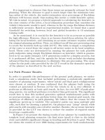
Fig. 5. Sydney Harbour bathymetric data. (a) The Harbour contains a number of interesting
features, including the Harbour tunnel on the right hand side and a number of large holes
which will present unique terrain signatures to the navigation filter. (b) The ship path for the
Sydney Harbour transect. Shown are the contours of the harbour together with the path of the
vehicle. Included in this data set are the GPS position and depth sounder observations at 5s
intervals.
5 Conclusions
The proposed terrain-aided navigation scheme has been shown to reliably track a ship
position in a harbour situation given depth soundings and a bathymetric map of the
harbour. This technique is currently being augmented to support observations using
a multi-beam or scanning sonar in preparation for deployment using the Unmanned
Underwater Vehicle Oberon available at the University of Sydney’s Australian Centre
for Field Robotics.
Following successful demonstration of the map based navigation approach, the
techniques developed will be applied to building terrain maps from the information
available solely from the vehicle’s on-board sensors. There is considerable informa-
tion contained in strong energy sonar returns received from the sea floor as well as
in the images supplied by on-board vision systems. This information can be com-
bined to aid in the identification and classification of natural features present in the
environment, allowing detailed maps of the sea floor to be constructed. These maps
can then be used for the purposes of navigation in a similar manner to that of the
more traditional, parametric feature based SLAM algorithm [13,12].
Acknowledgements
The authors wish to acknowledge the support provided under the ARC Centre of
Excellence Program by the Australian Research Council and the New South Wales
government. Thanks must also go to the staff of the Defence Science and Technology
Organization (DSTO) for making the Sydney Harbour bathymetry and transect data
available.
ATerrain-aided Tracking Algorithm for Marine Systems 101

(a) (b)
(c) (d)
Fig.6. Monte Carlo localisation example using the SydneyHarbour bathymetric map. The
line represents the ship track in this deployment and the particles are shown overlaid on the
figure. (a) The particles are initially drawn from the uniform distribution across the extent
of the harbour.(b) The potential location of the ship is reduced to areas of the harbour with
acommon depth to the start of the trial and (c) begin to convergeonthe true ship location.
(d) Once the particles have converged to the actual position of the ship, its motion is tracked
as additional observations are taken. As can be seen, the particle clouds track the true ship
path overthe extent of the run in spite of there being no absolute observations of the ship
position.
References
1. N. Bergman, L. Ljung, and F. Gustafsson. Terrain navigation using Bayesian statistics.
IEEE Control Systems Magazine,19(3):33–40, 1999.
2. F.
Gustafsson,
N. Bergman, U. Forssell, J. Jansson, R. Karlsson, and P-J Nordlund.
Pa
rticle filters for positioning,navigation andtracking.
IEEE
Tr
ans.
on Signal Processing,
1999.
3. A.E. Johnson and M. Hebert. Seafloormapgenerationforautonomousunderwater vehicle
navigation. Autonomous Robots,3(2-3):145–68, 1996.
4. D. Langer and M. Hebert. Building qualitative elveation maps from underwater sonar
data
for
autonomous

underw
ater
na
vigation.
In
Pr
oc.
IEEE
Intl.
Conf
.o
nR
obotics
and
Automation,volume 3, pages 2478–2483, 1991.
102 S. Williams and I. Mahon
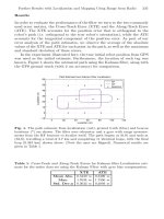
Fig.7. The error between the mean of the particle densities and the GPS positions.
The
errors are bounded by the 2
σ error
bounds for the distributions.
5. S. Majumder,S.Scheding, and H.F.Durrant-Whyte. Sensor fusion and map building
for underwater navigation. In Proc. Australian Conf.onRobotics and Automation,pages
25–30. Australian Robotics Association, 2000.
6.
C.
De
Moustier
and
H.

Matsumoto.
Seafloor
acoustic
remote
sensing
with
multibeam
echo-sounders and bathymetric sidescan sonar systems. Marine Geophysical Researches,
15(1):27–42, 1993.
7.
V.
Rigaud
and
L.
Marc
Absolute
location
of
underw
ater
robotic
ve
hicels
by
acoustic
data fusion. In Proc. IEEE Intl. Conf.onRobotics and Automation,volume 2, pages
1310–1315, 1990.
8. R.Karlsson, F. Gustafsson, and T. Karlsson. Particle filtering and cramer-rao lower bound
for underwater navigation. In Internal Report LiTH-ISY-R-2474,2002.
9. S. Thrun, D. Fox, and W. Burgard. Aprobabilistic approach to concurrent mapping and

localization for mobile robots. Machine Learning and Autonomous Robots (joint issue),
1998.
10. S. Thrun, D. Fox, W. Burgard, and F. Dellaert. Robust monte carlo localization for mobile
robots. Artificial Intelligence,2000.
11. L. Whitcomb, D. Yo erger,H.Singh, and J. Howland. Advances in underwater robot
vehicles for deep ocean exploration: Navigation, control and survey operations. The
Ninth Internation Symposium on Robotics Research,pages 346–353, 1999.
12. S.B. Williams, G. Dissanayake, and H.F.Durrant-Whyte. Constrained initialisation of
the simultaneous localisation and mapping algorithm. In Proc. Intl. Conference on Field
and Service Robotics,pages 315–320, 2001.
13. S.B. Williams, G. Dissanayake, and H.F.Durrant-Whyte. Towards terrain-aided naviga-
tion for underwater robotics. Advanced Robotics,15(5):533–550, 2001.
Experimental Results in Using Aerial LADAR Data
forMobile Robot Navigation
      
  
  

Abstract.            
           
              
               
               
           
                 
        
1Introduction
         
              
         

             
             
         
          
   
           
           
          
               
             
          
                
          
           
          
           
          
        
       
            
             


        
           
   ×             
          
           
              
         

            
              
            
           
      
2Data Sets
             
         
2.1 Data Collection
            
            
               
          
      
2.2 Sensors
            
           

             
             
             
           90
o
× 15
o

        ± 90
o
×±15
o

   
             
           
            
             
             
        
         
 
3Vegetation Filtering
              
            
           
       
3.1 Motivation
         
          
             
              
            
           
            
          
3.2 Vegetation and Active Range Sensors
            
          
  
          
            
         

       
           
             
            
           
            
              
            
               
            
            
              
  
3.3 State of the Art
           
           
        
          
         
          
             
         
            
            
    
3.4 Methods Implemented
           
            
          
  

Multi-echoes based filtering        
        ×      
            
             
           
           
            
               
              
               
    
Cone based filtering          
               
          
            
      
           
             
          
            
   ρ          
o

             

            
        ×     
   

4 Terrain Registration



          

4.1 Terrain Registration Method









 

10
o



























        
             
            
          
           
        
             

4.2 Example with the Yuma Data Set
Ledge course          
            
           
              
       ×            
         
      

Wash course           
             
           
               
              
           
           
   
             
             
             
           
            
              
 
           
            
       ×    ×      
            
   
5Path Planning
              
            
          

      
      
Fig.1.           
             
                

            
                 
             

5.1 Traversability Maps
             
          ×    
          
            
            vege-
tationess        
          
            
          
           45
o
               
             
           
         
            
             

        
              
      
5.2 Planner
            
               
C

comb.
( θ )=
1
(1 − C
trav.
( θ ))
2
+
1
(1 − C
veg.
)
2

 C
trav.
( θ )        θ    
       C
veg.
  vegetationess     
C
comb.
( θ )               

         vegetationess  
             
           
              
      vegetationess    
   vegetationess map    

            
             
             
            
     
           
                
             
          
5.3 Example with the APHill Data Set
            
           
             
         vegetationess
            
            
            
            
          
          
           
          
          
   

        
Fig.2.             
                
            
6Conclusion

               
        
          
          
            
            
             
         
           
         
        
            
            
         
          
            
            
Acknowledgments
        
           
       
References
          
ISPR Journal of Photogrammetry &Remote Sensing 

        
           
  IEEE International Conference on Robotics and Automation
           Interna-
tional Conference on Robotics and Automation

             
   IEEE Intelligent Vehicles Symposium
            Remote
Sensing and Reconstruction for Three-Dimensional Objects and scenes 
  
              
      International Archives of Photogrammetry
and Remote Sensing 
            
  Collaborative Technology Alliance Conference
             
            
IEEE Transaction on Geoscience and RemotreSensing     
            IEEE/RSJ Interna-
tional Conference on Intelligent Robots and Systems
            IEEE International
Conference on Computer Vision and Pattern Recognition
           IEEE Interna-
tional Conference on Computer Vision and Pattern Recognition
         Ph.D Thesis,
Carnegie Mellon University
             
   ISPRS Journal of Photogrammetry &Remote Sensing 
           
     Remote Sensing Environment 

              
International Archives of Photogrammetry and Remote Sensing  
             
    International Symposium on Experimental Robotics


              
           ISPRS Journal of
Photogrammetry and Remote Sensing
              SPIE
Aerosense Conference
            ISPRS workshop
on Land Surface Mapping and Characterization using laser altimetry
             Interna-
tioanl Symposium on Experimental Robotics


Autonomous Detection of Untraversability of the Path
on Rough Terrain forthe Remote Controlled Mobile
Robots
 
1
  
2
1
 

 
2
  


Abstract.             
               
               

             
               
                
             
       
1Introduction
            
            
            
            
             
               
   
         
             
     
           
        
2Traversability Test
           
   

           
   
      
Sensing plane
Map area
Test position
Fig.1.        
z

r
X
R
Y
R
Z
R
L
P
β
X
GL
Y
GL
Z
GL
z
s
x
s
Sensor
Sensing plane
x
r
y
r
α
Fig.2.  
             
   

           
             
       
            
           
           
    
2.1 Sensing Front
              
            
              
             
         

      X
GL
 Y
GL
 Z
GL
   
 X
R
 Y
R
 Z
R
          
 


( x
s
, 0 , z
s
) 
β L 
α 
( x
r
, y
r
, z
r
) 
( φ, θ, ψ ) 



P
X
GL
P
Y
GL
P
Z
GL


=


T
ij


L cos α
L sin α
1




T
11
= cos ψ cos θ cos β − sin β (sin ψ sin φ + cos ψ sin θ cos φ ) 
T
12
= − sin ψ cos φ + cos ψ sin θ sin φ 
T
13
= x
r
+ x
s
cos ψ cos θ + z
s
(sin ψ sin φ + cos ψ sin θ cos φ ) 

T
21
= sin ψ cos θ cos β
− sin β ( − cos ψ sinφ +sin ψ sinθ cos φ ) 
T
22
=cos ψ cos φ +sin ψ sinθ sin φ 
T
23
= y
r
+ x
s
sin ψ cos θ + z
s
( − cos ψ sin φ +sin ψ sin θ cos φ ) 
T
31
= − sin θ cos β − cos θ cos φ sin β 
T
32
=cos θ sin φ 
T
33
= z
r
− x
s
sin θ + z
s

cos θ cos φ 
          
         
    φ, θ, ψ        
           
            
   
2.2 Making Elevation Map
             
            
            
              
           
            
          
         
              
 
      
             
       
              

              
              

              

2.3 Test of Traversability
            

           
      
         
             
        
             
              
             
            
           
           
             
       H      
        
•     H         
    
•          
•               
                
    
Assumed position of Wheels
Examine point
Wheel
H : Height of the step
which wheel can pass over
Fig.3.      

Fig.4.        
Fig.5. 
•                

                
     
            
             
           
             
             
             
                 
                
      
3Implementation of Experimental System
3.1 Mobile Robot Platform "Yamabico-Navi"
          
      
        
 150mm       110mm    
450mm( W ) × 450mm( D ) × 700mm( H )      12kg

      
        
             
             
          
               
         
3.2 Sensing Front
Range measurement           
           
        

              
           ( x
c
,y
c
,z
c
)   
        θ
c
   
P          L    α   P
         
L =

x
2
+ y
2

α =tan
− 1
y
x

x =
z
c
tan(θ
c

− tan
− 1
v
F
)
+ x
c

y = h

x
2
+ z
2
c
F
2
+ v
2
+ y
c

 h  v            F  
        
        
x
s
=74 mm
z
s

=420mm
β =24 . 5 degree
x
c
= − 104mm
Fig.6.       

y
c
= 0 mm
z
c
= 168mm
θ
c
= 8 . 57degree
1 m 
1 cm 60cm
7 mm
Measurement of the robot posture 
t φ
( t )
, θ
( t )
, ψ
( t )

  ω
x ( t )
, ω

y ( t )
, ω
z ( t )

t + t 
φ
( t + ∆t)
=

ω
x ( t )
+

ω
y ( t )
sin φ
( t )
+ ω
z ( t )
cos φ
( t )

tan θ
( t )

t + φ
( t )

θ
( t + ∆t)

=

ω
y ( t )
cos φ
( t )
− ω
z ( t )
sin φ
( t )

t + θ
( t )

ψ
( t + ∆t)
=
ω
y ( t )
sin φ
( t )
+ ω
z ( t )
cos φ
( t )
cos θ
( t )
t+ ψ
( t )


 φ     θ     ψ      
  Z  Y  X         
           
            
         
Measurement of the robot position     
          
            
          
 
3.3 Making Elevation Map
          1 cm     
             
Fig.7.    

      
                 
   
        3 cm/second  
      1 cm    
3.4 Test of Traversability
         100mm   
            
             
            
         17mm      
  40mm
3.5 Remote Control of the Robot
            
          

              
              
           
   
4Experimental Results and Discussion
           
        A  E     F 
 
        A  E  
   F         
             A  E 

             
         X    
             
   
              
             
     
           
        
             
           
       

1100 207 197 546 207
207
100
1150
-100

-307
-397
197
494
297
X
Y
Height
A : 10 mm
B : 17 mm
C : 8 mm
D : 7 mm
E : 6 mm
F : 29 mm
AB
C
D
E
F
Fig.8.    
Fig.9.      
-4.5
-4
-3.5
-3
-2.5
-2
-1.5
-1
-0.5

0
0 200 400 600 800 1000 1200 1400 1600 1800 2000
Pitch [degree]
X [mm]
Fig.10.            
           
            
5Conclusion
           
           
            
         
           
          
         
     

      
Fig.11.      
References
           
       Journal of the Robotics Society of
Japan        
            
       International Conference on
Field and Service Robotics (FSR’97)    
              
         Proceedings of IEEE/RSJ
International Conference on Intelligent Robots and Systems(IROS) ‘91 
  

            
   Proceedings of IEEE/RSJ International Conference on
Intelligent Robots and Systems(IROS) ‘97    
        
  Proceeding of the 20th anual conference of RSJ  
  

×