Field and Service Robotics - Corke P. and Sukkarieh S.(Eds) Part 8 ppsx
Bạn đang xem bản rút gọn của tài liệu. Xem và tải ngay bản đầy đủ của tài liệu tại đây (3.27 MB, 24 trang )
247
Fig.1. Overviewofthe mechanism
Fig.2. Prototype Vehicle and Special wheel
2.2 Kinematics
The vehicle’sconfiguration, position and attitude are defined by the body parameters:
R1, R2 and wheel rotation velocity values ( ω
1
, ,ω
7
) ,inFigure 3.
Here, equation(1) indicates the wheel rotation velocity.
ω
i
= kV
i
( i =1, ,7) (1)
where,
r :radius of the wheel [mm]
ω
i
: rotation velocity of the wheel i [rad/s]
V
i
: rotation velocity of the actuator i [rad/s]
k :gear ratio between the actuator and the wheel
Now,
˙
X =
˙x ˙y
˙
θ
T
and V =
V
1
··· V
7
T
express the motion velocity vector
of the vehicle and the rotation velocity vector of the actuators, respectively. V is also
derivedbyusing
˙
X in equation (2).
V = J
+
·
˙
X, (2)
Development of a Control System of an Omni-directional Vehicle
248 D. Chugo et al.
where J
+
is pseudo inverse of Jacobian matrix;
J
+
=
J
T
J
− 1
J
T
=
1
kr
·
10R
2
0 − 1 R
1
− 10 R
2
100
10R
2
01R
1
− 10 R
2
(3)
Fig.3. Coordination and parameters
2.3 Problem Specification
The developed vehicle has redundant actuation system using sevenwheels. Thus,
our system has to synchronize the wheels with following each control reference,
which is calculated by equation (2) using Jacobian. However, during the robot passes
overthe irregular terrain, the load distribution to each wheel is complexproblem.
Therefore, it is difficult to synchronize among the wheel. If the system fails to take
the synchronization among the wheels, the vehicle will lose the balance of the body
posture as shown in Figure 4.
Thus, each wheel has to synchronize with the others when the vehicle runs on
the rough terrain. In related works, some traction control methods for single wheel
are already proposed. However, theydonot discuss synchronization of the wheels
for running on rough terrain. Forour system, we must consider the synchronization
among the wheels. We explain our proposed method in next section.
3 Control System
3.1 Proposed method
In order to synchronize the wheels rotation during the vehicle passes over the
step, calculated torque reference value should not over the maximum torque of the
249
Fig.4. The vehicle losing the balance
motor.Ifextraordinary load applies on the wheel(s) or the torque reference exceeds
maximum torque of the motor,the system cannot control the wheels, properly.
Our proposed control system is shown in Figure 5. The control reference is
calculated by PID-based control system (equation (4)).
Fig.5. Flowchart of the control system
The torque reference of i -motor is calculated by equation (4).
τ
i
= k
p
e + k
i
edt + k
d
de
dt
, (4)
where
e : Error value of the motor rotation velocity
k
p
: Proportional gain for PID controller
k
i
: Integral gain for PID controller
k
d
: Derivative gain for PID controller
Development of a Control System of an Omni-directional Vehicle
250 D. Chugo et al.
The coefficient k
i
is calculated as:
k
i
=
τ
max
τ
i
if τ
i
> τ
max
,
1 if τ
i
≤ τ
max
,
(5)
where
τ
max
: Maximum torque of the motor
τ
i
: Calculated torque value
i : 1 . . . 7 (number of an actuator)
The reference torque is determined by equation (6):
τ
out
i
= k × τ
i
, (6)
where k = min { k
1
, ···, k
7
} .
The controller adjusts the synchronization among the wheel in the case of ex-
traordinary load occurring.
3.2 Simulation
We verify the performance of our method by computer simulations. As initial
conditions, three motors are rotating at same fixed velocity speed 100[deg/s] and the
load applies to each motor independently. The load is approximated by a dumper
model and the dumper coefficients are applied to each wheel as follows.
load A : 0.001[Nm/deg] from 37 to 60[sec]
load B : 0.004[Nm/deg] from 14 to 52[sec]
load C : 0.005[Nm/deg] from 22 to 57[sec]
In this case, we assume that the maximum torque of the motor is 30[N].
The results of the simulation are shown in Figure 6. During the load applied
to the wheel (from 14 to 60[sec]), rotation velocity of the motor is reduced. Using
proposed method, each controller adjusts control command to the wheel and recovers
synchronization among the wheel.
3.3 Method of Sensing the Step
We utilized PID based control system, however it is difficult to determine the
parameters of the controller when the control target has complex dynamics. Thus, we
switch two parameter sets according to the situations. The vehicle has the accurate
control mode for the flat floor and the posture stability control mode for the rough
terrain. The stability mode utilizes the proposed traction control method, too.
251
Fig.6. Simulation result
In order to switch twoparameter sets, the terrain estimation function is required.
Thus, we proposed the estimation method using the body axes. The angle of two
axes of the body is changed passively by the ground surface. The terrain can be
measured by using the body kinematics information. Twopotentiometers measure
the angle of the axes (Figure 7). By this information, the controller can switch two
parameter sets according to the terrain condition.
Fig.7. TwoPotentiometers
4 Experiment
Here, we have the following two experiments.
Development of a Control System of an Omni-directional Vehicle
252 D. Chugo et al.
4.1 Measuring the Step
In first experiment, we verify the sensing ability of the vehicle when it passes over
the rough ground. The vehicle climbs the step with 30[cm] depth and 1[cm] height.
The experimental result is shown in Figure 8 and it indicates that the height of
the step is 0.9[cm] and the depth is 32.5[cm]. Our vehicle need to change the control
mode when the step is more than 3[cm] [7], it is enough step detection capability.
Fig.8. The result of measuring the step
4.2 Passing Over the Step
Second experiment is for passing over the steps. The vehicle moves forward at
0.3[m/s] and passes over the 5[cm] height step. Furthermore, we compare the result
by our proposed method with the one by general PID method.
As the result of this experiment, the vehicle can climb up the step more smoothly
by our method (Figure 9). The white points indicate the trajectory of the joint point
on the middle wheel and they are plotted at every 0.3 [sec] on Figure 9.
Figure 10 and 11 show the disturbed ratio which means the error ratio of the
rotation velocity (a), the slip ratio (b) [11] and the rotation velocity of each wheel
(c). The disturbed rotation ratio and the slip ratio are defined by the equation (5) and
the equation (6), respectively.
ˆ
d =
ω
ref
− ω
ω
(7)
ˆs =
rω − v
ω
rω
(8)
ω : Rotation speed of the actuator.
ω
ref
: Reference of rotation speed.
r :The radius of the wheel.
v
ω
: The vehicle speed.
As the result, the rotation velocity of the wheels is synchronized with the pro-
posed control method. Furthermore, the disturbed rotation ratio and the slip ratio are
reduced. Thus, this control method is efficiencyfor step climbing.
253
Fig.9. Step climbing with proposed controlling and general controlling
(a)The disturbed rotation ratio
(b)The slip ratio
(c)The rotation speed
Fig.10. Experimental Result of proposed method
(a)The disturbed rotation ratio
(b)The slip ratio
(c)The rotation speed
Fig.11. Experimental Result of old method
Development of a Control System of an Omni-directional Vehicle
254 D. Chugo et al.
5Conclusions
In this paper,wediscuss the control method for omni-directional mobile vehicle
with step-climbing ability and the terrain estimation method using its body.Wealso
designed newcontrol system which realized the synchronization among the wheels
when the vehicle passed overrough terrain.
We implemented the system and verified its effectiveness by the simulations and
experiments. Forfuture works, we will consider the motion planning method based
on the environment information.
References
1. G. Campion, G. Bastin and B.D. Andrea-Novel, “Structual Properties and Classification
of Kinematic and Dynamic Models of Wheeled Mobile Robots,” IEEE Transactions on
Robotics and Automation,vol. 12, No. 1, pp. 47–62, 1996.
2. G. Endo and S. Hirose, “Study on Roller-Walker: System Integration and Basic Ex-
periments,” IEEE Int. Conf on Robotics &Automation,Detroit, Michigan, USA, pp.
2032–2037, 1999.
3. M. Wada and H. Asada, “Design and Control of aVariable Footpoint Mechanism for
Holonomic Omnidirectional Vehicles and its Application to Wheelchairs,” IEEE Trans-
actions on Robotics and Automation,vol. 15, No. 6, pp. 978–989, 1999.
4. S. Hirose and S. Amano, “The VUTON: High Payload, High EfficiencyHolonomic
Omni-Directional Vehicle,” 6th Int. Symposium on Robotics Research,Hidden Valley,
Pennsylvania, USA, pp. 253–260, 1993.
5. A. Yamashita, et.al.,“Development of astep-climbing omni-directional mobile robot,”
Int. Conf.onField and Service Robotics,Helsinki, Finland, pp. 327–332, 2001.
6. K.Iagnemma, et.al.,“Experimental Validation of Physics-Based Planning and Control
Algrithms for Planetary Robotic Rovers,” 6th Int. Symposium on Experimental Robotics,
Sydney, Australia, pp. 319–328, 1999.
7. K.Yoshida and H.Hamano, “Motion Dynamic of aRoverWith Slip-Based Traction
Model,” IEEE Int. Conf on Robotics &Automation,Washington DC, USA, pp. 3155–
3160, 2001.
8. H. Asama, et.al.,“Development of an Omni-Directional Mobile Robot with 3DOF
Decoupling Drive Mechanism,” IEEE Int. Conf on Robotics &Automation,Nagoya,
Japan, pp. 1925–1930, 1995.
9. T. Estier, et.al.,“An Innovative Space Roverwith Extended Climbing Abilities,” Video
Proc. of Space and Robotics 2000,,Albuquerque, NewMexico, USA, 2000.
10. (as of Nov. 2003)
11. D. Chugo, et.al.,“Development of Omni-Directional Vehicle with Step-Climbing Abil-
ity,” IEEE Int. Conf on Robotics &Automation,Taipei, Taiwan, pp. 3849–3854, 2003.
Sensor-Based Walking on Rough Terrain
for Legged Robots
1
1
1
1
2
1
2
Abstract.
1 Introduction
256 Y. Mae et al.
Fig.1. Alimb mechanism robot. Fig.2. Radial arrangementoflimbs.
keeping its stability.Alimb mechanism robothas been designed and developed
taking such omnidirectional mobility into account[14].
As one of feasible structures of the limb mechanism a6-limb mechanism has
been
analyz
ed
and
eva
lu
ated
in
the
aspects
of
omn
idirection
al
mobility
[15
,16].
In
[15,16], twotypes of structures are compared with respect to their stroke, stability,
and errorofdead reckoning for six-legged locomotion. The radial legarrangement
model
will
be
pro
ve
dt
oh
av
eh
igher
omnidir
ectional
mobility
than
the
para
llel
le
g
arrangement.
In actual tasks it is essential for alimb mechanism robottomoveonrough
terrains quickly andsmoothly.Furthermore,inmanipulationtasks, alimbmechanism
robothas to select adequate footholds of supporting limbs not to fall down due to
manipulation motionsoflimbs.
In the presentpaper,first we introduce alimb mechanism robot, and describe
mainly followingtwo topics. one is asimple trajectory generation methodincon-
sidering gait controlstrategy on the unevenground. It can maintain the walking
speed of the robotwhile keeping high stability,evenwhen atransfer limb lands on a
bump. The other is adjustment of footholds of four supporting limbs from the point
of viewofstatic stability.The footholds should be selected to keep higher stability
marginwhen twolimbs are used as manipulation. In the paper,weexamine the case
twoneighboring limbs are used as arms, which makes the limb mechanism robot
unstable the most.
2Limb Mechanism Robot
2.1 Configuration of Limb Mechanism Robot
First, we introduce alimb mechanism robotdeveloped by Takahashi et al.[14,15]
(see Fig.1). In designing,the main concern is to fix the number of limbs. Afour
limb mechanism will be feasible, butits mobility is extremely limited while one of
limbs will be employed for arm function.Too manylimbs, for example sevenor
Sensor-Based Walking on Rough Terrain for Legged Robots 257
Fig.3. Configuration of alimb.
more, may cause difficulty in gait control. Asix limb mechanism seems the most
reasonable in the aspects of achievinghigh mobility and manipulability,since it
enables four-legged locomotion with twoarm manipulation in addition to six-legged
locomotion.
Arrangement of limbs are importantparameter to determine property of alimb
mechanism robot. In most insects, twogroupsofthree legs are arranged in parallel.
This parallel arrangement has strong directivity in walking and working capabilities.
No directivity,oromnidirectional mobility,may be preferable when the robotisap-
plied
in
an
arro
we
nv
iro
nment
where
postur
ea
nd
rotatio
nal
motion
sa
re
constrained
.
Especially in roughterrains, omnidirectionalmobility is useful to obtain stable and
quick
change
of
wa
lking
directions.
If
six
le
gs
are
arran
ged
equally
or
equilaterally
,
then the directivity and the interference amonglegscan be improvedand alarge
workingspace can be assured for each limb.
Thus, the limb mechanism robot has been developed to have six limbs which are
arranged radially (see Fig.2). Each limb has a3d.o.f. serial linkage.The structure is
arotation-pivot-pivotarticulation as shown in Fig.3. We call the joints first, second,
and third joints in orderfrom the body to the end.
2.2 OverviewofControl System
In outdoor working,remote control is desirable because controlcables disturb a
robo
tt
ow
ork
smooth
ly
.S
ince
the
de
ve
lo
ped
limb
mecha
nism
robo
th
as
18
d.o.f
.,
calculation of the amount of controlofeach actuatorinthe whole generation of
operation becomes very complicated. Although what has ahighly efficient computer
for control is required, such acomputer cannot be carried in amain part from
the point of asize and weight, and sufficient calculation cannotbeperformed by
computer which can be conversely put on amain part.
Thusweadoptaradio controlsystem. Figure 4shows the overviewofthe whole
system.
This
system
consists
of
at
ransmitter
,a
recei
ve
r,
and
serv
omoto
rs.
The
trans-
mitter is connected with the controlcomputer.Wecan drive the servomotors in
proportion to the position commands which we inputtothe computer.The servomo-
tors of the robot are controlled in open loop.The robot is equipped with the sensor
module. It is constituted by an acceleration sensor,aPIC(a small CPU with A/D
converter), and atransmitter.The PIC processes the sensed gravity to obtain inclina-
258 Y. Mae et al.
Fig.4. Overviewofthe control system.
tion of the body and transmits it to the PC. The PC generates the motion pattern of
the robot and transmites the corresponding position commands to the servomotors.
3 Basic Walking Trajectory
3.1 Simplified Trajectory Generation
As indicated in the previous discussion, it is rather complicated and tiresome to
find the trajectory of each leg for the generation of the gait pattern. A more general
treatment will be considered to find unique trajectory in any directions in each limb.
The method is simple and easy to generate trajectories with the same stroke in any
directions.
Figure 5 shows one example of the largest size of a circled area in the working
space of the limb. Any linear trajectories will be possible in any directions within it,
therefore the trajectory generation for each limb might become much easier both in
four and six-legged locomotion. A control software is implemented in the controller
PC. Actual omnidirectional walking motion has been confirmed in the developed
robot.
The diameter of the circle is determined from the workspace of a limb. Figure 6
shows sectional view of the workspace of a limb. The workspace is between outer
curved line and inner curved line. We assume a cylinder inscribed in the workspace
to generate basic trajectory of a limb (see Fig.6). Then observe two perimeters of
circles and draw two perpendiculars from perimeters’ end to end. These lines make
the basic trajectory.
The method makes it possible to make the stroke of limbs the same length as
every direction. The stroke is diameter of a circle. Usually on regular terrains, the end
of limb passes on this trajectory. The trajectory consists of four terms, lift up, forward
motion, landing, and backward motion. They are shown in Fig.7(a). As shown in
Fig.7(b), in case of changing moving direction of the robot, simple rotation of the
Sensor-Based Walking on Rough Terrain for Legged Robots 259
Fig.5. Strokeinomnidirectional locomotion.
Fig.6. Cylinder inscribed in workspace.
(a) Regular trajectory. (b) Trajectory in changing
moving direction.
Fig.7. Basic trajectory of alimb.
trajectory
mak
es
omnid
irectional
locom
otion
easy
,w
hereby
the
limb
mech
anism
robo
tc
an
chang
et
he
mo
vi
ng
direction
without
re-stepp
ing.
3.2 Simplified Gait PatternbyPhase Shift
Legmechanisms likeinsects or animals have symmetry in longitudinal and lateral
directions, thus their stability marginand strokevaries in 90[deg.] phase, or it
may be called four axes symmetry. In the gait controlthe trajectoryofeach leg
may be generated only for this phase, and it can be repeatedly used in the other
directionsbytaking this symmetry into account. In our limb mechanism robotthe
trajectories in 60[deg.] phase can be repeated due to its six axes symmetry. This may
allo
ws
simpler
contro
ls
trate
gy
ev
en
in
fou
r-
le
gged
gait
as
well
as
in
six-le
gg
ed.
The
omnidirectional gait may be generated simply by switching the basic gait patterns
six times. Furthermore, the patternshas symmetry centred in one limb, thus theyare
again reduced to ahalf, that is, the trajectoriesin 30[deg.] phase are only required
for the gait control.
260 Y. Mae et al.
Fig.8. Trajectory on abump. Fig.9. Pose adjustment to reduce inclination of the body.
Fig. 10. Limb mechanism robot on a bump with pose adjustment.
4 Sensor-Based Waling on Rough Terrain
On bumpy or rough terrains, it is difficult for the robot to continue walking by the
basic trajectory described in the previous section. When some limbs land to bumps
or into hollows, the body inclines and it reduces stability margin. In the worst case,
the robot falls down. Thus, it is necessary to adjust the pose of the body in walking
on the uneven ground.
Easy conversion of the basic trajectory should make the robot possible to walk-
ing on the uneven ground while keeping omnidirectional mobility. We describe a
trajectory generation method for walking on the uneven ground, which uses an ac-
celeration sensor attached to the body to measure the inclination of the body. In
the sensor-based trajectory generation, the following process is added to the basic
trajectory generation process.
If the inclination is detected in "landing" term, the landing motion of the limb is
stopped and the supporting limbs are moved to reduce the inclination. After adjusting
inclination, some ends of limbs may reach the end of working space and cannot move
any more. Then, in order to bring the ends of the limb into the working space and
keep the height of the body constant, all landing limbs should be folded as shown
in Fig.9. After folding landing limbs, the landing limb performs backward motion.
Though there are differences of levels between landing positions of limbs, the robot
can continue to move by adjusting verical trajectory length of the limbs.
In this way, the robot walks on the uneven ground while keeping high stability
margin. Figure 10 shows a scene where the robot moves over a bump in the tripod
gait using six limbs. The sensor-based pose adjustment algorithm is implemented
Sensor-Based Walking on Rough Terrain for Legged Robots 261
Fig.11. Change of stabilty marign while walking on the unevenground.
in the walking algorithm. We can see the pose of the body is kept horizontally by
reducing inclination even alimb is on abump.
The left and right figures in Fig.11 showthe changes of stability marginwithout
and with the pose adjustmentinwalking, respectively.The horizontal axes indicate
the walking distance of the robot. The vertical axes indicate stability margin. The
circle in the left figure indicates the part where the limb lands on abump and the sta-
bility margindecreases. In the right figure,the stability marginatthe corresponding
part doesnot decrease. From the figures, we can see the adjustmentofthe pose of
the bodymakes stability marginalmost constant even the robotmovesoverabump.
5Adjustment of Footholds of Supporting Limbs
To keep static stability in manipulation tasks, the robothas to adjust footholds of
suppo
rting
limbs
in
accord
ance
with
the
pose
of
the
manipu
lation
limbs.
We
discuss
adjusting footholds of supporing limbs in the case that the twoneighboringlimbs
are used as arms. This is the case that the mass center of the robotchanges the most.
The
side
of
the
manip
ulation
limbs
is
called
front
or
for
wa
rd,
tempo
rarily
.F
igure
12
shows alimb mechanism adjusting footholds of supporting limbs; twoneighboring
limbs are lifted up in parallel in frontofthe robot for simulation of manipulation
by twoneighboring limbs. When the robotmoves the twoneigboring limbs up, the
robotfalls down if it does not adjust the footholds of supporting legs.
We examinethe change ofstability margin dependingonthefootholdsofsupport-
ing
limbs.
In
the
ex
amina
tion,
we
fix
the
heigh
to
ft
he
body
to
149[mm] hor
izontally
by
fixing
the
joints
of
suppor
ting
limbs.
In
that
pose,
the
second
joint
is
at
60 de
gr
ees
downward and the third joint is at 0 degrees. Only the first joints of supporting limbs
are rotated to changethe footholds.
Figure13shows the changeofstability marginwhen the twofirst joints of the
frontside supporting limbs are rotated from 0 degrees to 60 degrees in forward
262 Y. Mae et al.
Fig
.1
2.
Al
imb
mechainism
robot
suppo
rted
by
four
limbs
while
tw
on
eighboring
limbs
are
lifted up.
Fig.13. Change of stability margin for changingfootholds by rotating the first joints of the
front side limbs.
direction,while the twoneighboring limbs are lifted up in parallel. When the first
joints are set at 0 degrees, the limbs are set at standard pose where the limbs are
spread radially.The horizontal axis indicates the sum of the rotational angles of
the twojoints. The vertical axis indicates stability margin. As the limbs are moved
forward, stability marginisincreased monotonously.The maximum stability margin
is obtainedatthe limit of the rotational angles 60 degrees. Thus, the twofrontside
suppo
rting
limbs
should
be
mo
ve
df
orw
ard
to
obtain
maximu
ms
tability
mar
gi
n
beforetwo neighboring limbs are movedupfor manipulation.
Figure14shows the changeofstability marginwhen the twoneighboring limbs
are beingupinparallel, while the twofirst joints of the front side supporting limbs
are
at
60 de
gr
ees
in
forw
ar
dd
irection.
The
tw
on
eigh
boring
manip
ulation
limbs
are
mo
ve
du
pb
ya
ctuating
second
and
third
joints.
The
horiz
ontal
axis
indica
tes
the
sum
Sensor-Based Walking on Rough Terrain for Legged Robots 263
Fig.14. Change of stability margin for moving twoneighboring limbs after adjusting the
footholds to maximize stability margin.
of the rotational angles of the twojoints. The vertical axis indicates stability margin.
We examine twomotion pattern of moving limbs. In the first pattern, the third joint
is
actuated
first
and
the
second
joint
is
actuated
ne
xt
(motion
Ai
nF
ig.14).
In
the
second pattern, the second joint is actuated first and the third joint is actuated next
(motionBinFig.14). The second joint is rotated upward from − 60 degrees to 45
degrees. The third joint is rotated upwardfrom 0 degrees to 90 degrees.
From Fig.14 we can see the high stability marginishold for the twomotion
patterns. This is because the footholds of the frontside supporting limbs are adjusted
to increase stability margin,before movingtwo neighboring manipulation limbs.
6Conclusions
In the paper,first we introduced amobile robotwith limb mechanism, and abasic
trajectory generation for omnidirectionallocomotion. Second, we describeasensor-
based walking method on rough terrains using an acceleration sensor attached to
the body.The experimental results of walking on the unevenground showthe pose
of the bodyiskept horizontally constant when alimb of the robot is on abump in
walking. Third,wedescribe adjustmentoffootholds of supporting limbs to keep
high stability marginwhile twoneighboring limbs are used as arm. The change of
stability marginisexamined in accordance with the change of the footholds.
Acknowledgement
This research wasperformed as apart of Special Project for EarthquakeDisaster
Mitigation in Urban Areas in cooperation with International Rescue System Institute
(IRS) and National Research Institute for Earth Science and Disaster Prevention
(NIED).
264 Y. Mae et al.
References
1. G.Pritschow, et.al., "Configurable Control System of aMobile Robot for On-site Con-
struction Masonry," Proc. of 10th Inter.Symposium on Robotics and Automation in
Construction,
pp.85
–92,
1993.
2. E.Papadopoulos and S.Dubowsky, "On the Nature of Control Algorithms for Free-
Floating Space Manipulators," IEEE Transaction on Robotics and Automation, vol.7,
no.6,
pp.759
–770,
1991
.
3. E.Nakano, et al., "First Approach to the Developmentofthe Patient Care Robot," Proc.
11th Inter.Symposium on Industrial Robot, pp.87–94, 1981.
4.
S.Skaar
,e
t.al.,
"Nonho
lonomic
Camera-Space
Manipu
lation",
IEEE
Tr
ansaction
on
Robotics and Automation, vol.8, no.4, pp.464–479,1992.
5. Y.F.Zheng and Q.Yin, "Coordinating Multi-limbed Robot for Generating Large Cartesian
Force," Proc. of IEEE Inter.Conf. on Robotics and Automation, pp.1653–1658,1990.
6. C.Su and Y. F. Zheng, "Task Decomposition for aMulti-limbed Robot to Work in Reach-
able But Unorientable Space," IEEE Transaction on Robotics and Automation, vol.7,
no.6, pp.759–70, 1991.
7. S.Sugiyama, et.al., "Quadrupedal Locomotion Subsystem of Prototype AdvancedRobot
for Nuclear Power plant Facilities," Proc. of Fifth Inter.Conf. on Advanced Robotics,
pp.326–333, 1991.
8. K.Hartikainen, et al., "Control and Software Structures of aHydraulic Six-Legged Ma-
chine Designed for Locomotion in Natural Environments," Proc. of IEEE/RSJInter.
Workshop on Intelligent Robots and Systems, pp.590–596, 1996.
9. N.Koyachi, et al., "Integrated Limb Mechanism of Manipulation and Locomotion For
Dismantling Robot -Basic concept for control and mechanism -,"Proc. of the 1993
IEEE/TsukubaInter.Workshop on Advanced Robotics, pp.81–84, 1993.
10. N.Koyachi, et al., "Hexapod with Integrated Mechanism of Legand Arm," Proc. of IEEE
Inter.Conf. on Robotics and Automation, pp.1952–1957, 1995.
11. T.Arai, et al., "Integrated Arm and LegMechanism and its Kinematics Analysis," Proc.
of IEEE Inter.Conf. on Robotics and Automation, pp.994–999,1995.
12. N.Koyachi, et al., "Design and Control of Hexapod with Integrated Limb Mechanism:
MELMANTIS,"
Proc.
of
1996
IEEE/RS
JI
nter
.C
onf.
on
Intelligent
Robots
and
Systems,
pp.877–882, 1996.
13. J.Racz, et al., "MELMANTIS -the Walking Manipulator," Proc. of the 5th Inter.Sym-
posium
on
Intelligent
Robotic
Systems,
pp.23–2
9,
1997
.
14. Y.Takahashi, et al., "Development of Multi-Limb Robot with Omnidirectional Manipu-
lability and Mobility," Proc. of 2000 IEEE/RSJ Inter.Conf. on Intelligent Robots and
Systems, pp.877–882,2000.
15.
T.
Arai,
et
al.,
“Omni-Directional
Mobility
of
Limb
Mech
anism
Robot,
”P
roc.
of
4th
Inter
.
Conf. on Climbing and Walking Robots, pp.635–642,2001.
16. Y.Mae, et al., “Evaluation of omni-directional mobility of multi-legged robots based on
error analysis of dead reckoning,”Proc. of 5th Inter.Conf. on Climbing and Walking
Robots,
pp.271
–278,200
2.
Experiments in Learning Helicopter Control
from a Pilot
1 , 2
1
2
1
2
Abstract.
1Introduction
Fig.1.
2Approach Outline
ψ φ θ
[ v, φ ] [ Z, w ]
δ
lat
δ
lon
δ
tail
3Platform Description
[ uvw ] [ pqr ] [ φθψ ]
ψδ
tail
φ
v
col
δ
lon
δ
lat
δ
lat
δ
w
Z
φ
θ
Learning
Controller
Learning
Controller
Learning
Controller
Learning
Controller
Learning
Controller
Fig.2.
[ XY Z ] δ
lat
δ
lon
δ
tail
δ
col
4Learning Control Structure
µ
Ai
µ
Bj
A i B j
C
ij
M
ij
C
ij
= µ
Ai
µ
Bj
o =
i
j
C
ij
y
ij
i
j
C
ij
y
ij
M
ij
δ
[ x
t
,δ
t
]
¯
M
ij
t
maxC
ij
∀ i, j | x
t
¯y
ij
δ
t
,
¯
C
ij
t
x
t
¯
M
ij
t
¯y
ij
=
t
δ
t
¯
C
ij
t
t
¯
C
ij
t
N
N =1
5Learnt Controller Performance
5.1 Heading Control
200 220 240 260 280 300
100
120
140
160
180
200
Time (seconds)
ψ (degrees)
Heading control − real helicopter flight
demand
response
−100 −80 −60 −40 −20 0 20 40 60 80 100
0.4
0.45
0.5
0.55
0.6
0.65
0.7
0.75
FAM surface for heading control − real helicopter flight
ψ (degrees)
δ
tail
Fig.3.
5.2 Roll Control
5.3 Pitch Control
5 / 8
221 222 223 224 225 226 227 228 229
−4
−2
0
2
4
6
Time (seconds)
φ (degrees)
Roll tracking
demand
response
−5 −4 −3 −2 −1 0 1 2 3 4 5
0.52
0.54
0.56
0.58
0.6
0.62
0.64
φ (degrees)
δ
lat
FAM surface for roll control
Fig.4.
194 196 198 200 202 204 206
−6
−4
−2
0
2
4
Time (seconds)
θ (degrees)
Pitch tracking
demand
response
Fig.5.
5.4 Height Control