Rapid Learning in Robotics - Jorg Walter Part 4 pdf
Bạn đang xem bản rút gọn của tài liệu. Xem và tải ngay bản đầy đủ của tài liệu tại đây (224.73 KB, 16 trang )
3.5 Strategies to Avoid Over-Fitting 35
could be extracted from a sequence of three-word sentences (Koho-
nen 1990; Ritter and Kohonen 1989). The topology preserving prop-
erties enables cooperative learning in order to increase speed and ro-
bustness of learning, studied e.g. in Walter, Martinetz, and Schulten
(1991) and compared to the so-called Neural-Gas Network in Walter
(1991) and Walter and Schulten (1993).
The Neural-Gas Network shows in contrast to the SOM not a fixed
grid topology but a “gas-like”, dynamic definition of the neighbor-
hood function, which is determined by (dynamic) ranking of close-
ness in the input space (Martinetz and Schulten 1991). This results in
advantages for applications with inhomogeneous or unknown topol-
ogy (e.g. prediction of chaotic time series like the Mackey-Glass
series in Walter (1991) and later also published in Martinetz et al.
(1993)).
The choice of the type of approximation function introduces bias, and
restricts the variance of the of the possible solutions. This is a fundamental
relation called the bias–variance problem (Geman et al. 1992). As indicated
before, this bias and the corresponding variance reduction can be good or
bad, depending on the suitability of the choice. The next section discusses
the problem over-using the variance of a chosen approximation ansatz,
especially in the presence of noise.
3.5 Strategies to Avoid Over-Fitting
Over-fitting can occur, when the function gets approximated in the do-
main , using only a too limited number of training data points .If
the ratio of free parameter versus training points is too high, the approxi-
mation fits to the noise, as illustrated by Fig. 3.4. This results in a reduced
generalization ability. Beside the proper selection of the appropriate net-
work structure, several strategies can help to avoid the over-fitting effect:
Early stopping: During incremental learning the approximation error is
systematically decreased, but at some point the expected error or
lack-of-fit starts to increase again. The idea of early stop-
ping is to estimate the on a separate test data set and de-
termine the optimal time to stop learning.
36 Artificial Neural Networks
X
X
Figure 3.4: (Left) A meaningful fit to the given cross-marked noisy data. (Right)
Over-fitting of the same data set: It fits well to the training set, but is performing
badly on the indicated (cross-marked) position.
More training data: Over-fitting can be avoided when sufficient training
points are available, e.g. by learning on-line. Duplicating the avail-
able training data set and adding a small amount of noise can help
to some extent.
Smoothing and Regularization: Poggio and Girosi (1990) pointed out that
learning from a limited set of data is an ill-posed problem and needs
further assumptions to achieve meaningful generalization capabili-
ties. The most usual presumption is smoothness, which can be formal-
ized by a stabilizer term in the cost function Eq. 3.1 (regularization
theory). The roughness penalty approximations can be written as
argmin (3.7)
where is a functional that describes the roughness of the func-
tion . The parameter controls the tradeoff between the fi-
delity to the data and the smoothness of . A common choice for
is the integrated squared Laplacian of
(3.8)
which is equivalent to the thin-plate spline (for ; coined by the
energy of a bended thin plate of finite extent). The main difficulty is
the introduction of a very influential parameter and the computa-
tion burden to carry out the integral.
For the topology preserving maps the smoothing is introduced by
a parameter, which determines the range of learning coupling be-
3.6 Selecting the Right Network Size 37
tween neighboring neurons in the map. This can be interpreted as a
regularization for the SOM and the “Neural-Gas” network.
3.6 Selecting the Right Network Size
Beside the accuracy criterion ( , Eq. 3.1) the simplicity of the network
is desirable, similar to the idea of Occam's Razor. The formal way is to
augment the cost function by a complexity cost term, which is often written
as a function of the number of non-constant model parameters (additive
or multiplicative penalty, e.g. the Generalized Cross-Validation criterion
GCV; Craven and Wahba 1979).
There are several techniques to select the right network size and struc-
ture:
Trial-and-Error is probably the most prominent method in practice. A
particular network structure is constructed and evaluated, which in-
cludes training and testing. The achieved lack-of-fit ( ) is esti-
mated and minimized.
Genetic Algorithms can automize this optimization method, in case of a
suitable encoding of the construction parameter, the genome can be
defined. Initially, a set of individuals (network genomes), the pop-
ulation is constructed by hand. During each epoch, the individuals
of this generation are evaluated (training and testing). Their fitnesses
(negative cost function) determine the probability of various ways of
replication, including mutations (stochastic genome modifications)
and cross-over (sexual replication with stochastic genome exchange).
The applicability and success of this method depends strongly on
the complexity of the problem, the effective representation, and the
computation time required to simulate evolution. The computation
time is governed by the product of the (non-parallelized) population
size, the fitness evaluation time, and the number of simulated gen-
erations. For an introduction see Goldberg (1989) and, e.g. Miller,
Todd, and Hegde (1989) for optimizing the coding structure and for
weights determination Montana and Davis (1989).
Pruning and Weight Decay: By including a suitable non-linear complex-
ity penalty term to the iterative learning cost function, a fraction of
38 Artificial Neural Networks
the available parameters are forced to decay to small values (weight
decay). These redundant terms are afterwards removed. The disad-
vantage of pruning (Hinton 1986; Hanson and Pratt 1989) or optimal
brain damage (Cun, Denker, and Solla 1990) methods is that both start
with rather large and therefore slower converging networks.
Growing Network Structures (additive model) follow the opposite direc-
tion. Usually, the learning algorithm monitors the network perfor-
mance and decides when and how to insert further network elements
(in form of data memory, neurons, or entire sub-nets) into the ex-
isting structure. This can be combined with outliers removing and
pruning techniques, which is particularly useful when the grow-
ing step is generous (one-shot learning and forgetting the unimpor-
tant things). Various unsupervised algorithms have been proposed:
additive models building local regression models (Breimann, Fried-
man, Olshen, and Stone 1984; Hastie and Tibshirani 1991), dynamic
memory based models (Atkeson 1992; Schaal and Atkeson 1994),
and RBF net (Platt 1991); the tiling algorithm (for binary outputs;
Mézard and Nadal 1989) has similarities to the recursive partition-
ing procedure (MARS) but allows also non-orthogonal hyper-planes.
The (binary output) upstart algorithm (Frean 1990) shares similarities
with the continuous valued cascade correlation algorithm (Fahlman
and Lebiere 1990; Littmann 1995). Adaptive topological models are
studied in (Jockusch 1990), (Fritzke 1991) and in combination with
the Neural-Gas in (Fritzke 1995).
3.7 Kohonen's Self-Organizing Map
Teuvo Kohonen formulated the (Self-Organizing Map) (SOM) algorithm as
a mathematical model of the self-organization of certain structures in the
brain, the topographic maps (e.g. Kohonen 1984).
In the cortex, neurons are often organized in two-dimensional sheets
with connections to other areas of the cortex or sensor or motor neurons
somewhere in the body. For example, the somatosensory cortex shows a
topographic map of the sensory skin of the body. Topographic map means
that neighboring areas on the skin find their neural connection and rep-
resentation to neighboring neurons in the cortex. Another example is the
3.7 Kohonen's Self-Organizing Map 39
retinotopic map in the primary visual cortex (e.g. Obermayer et al. 1990).
Fig. 3.5 shows the basic operation of the Kohonen feature map. The
map is built by a
(usually two) dimensional lattice of formal neurons.
Each neuron is labeled by an index
, and has reference vectors
attached, projecting into the input space (for more details, see Kohonen
1984; Kohonen 1990; Ritter et al. 1992).
w
a
x
Array of
Neurons
a
*
a
*
Input Space
X
Figure 3.5: The “Self-Organizing Map” (“SOM”) is formed by an array of pro-
cessing units, called formal neurons. Here the usual case, a two-dimensional array
is illustrated at the right side. Each neuron has a reference vector
attached,
which is a point in the embedding input space
. A presented input will se-
lect that neuron with
closest to it. This competitive mechanism tessellates the
input space in discrete patches - the so-called Voronoi cells.
The response of a SOM to an input vector is determined by the ref-
erence vector of the discrete “best-match” node . The “winner”
neuron is defined as the node which has its reference vector closest
to the given input
argmin (3.9)
This competition among neurons can be biologically interpreted as a result
of a lateral inhibition in the neural layer. The distribution of the reference
vectors, or “weights” , is iteratively developed by a sequence of training
vectors . After finding the best-match neuron all reference vectors are
40 Artificial Neural Networks
updated by the following adaption rule:
(3.10)
Here
is a bell shaped function (Gaussian) centered at the “win-
ner”
and decaying with increasing distance in the neuron layer.
Thus, each node or “neuron” in the neighborhood of the “winner” par-
ticipates in the current learning step (as indicated by the gray shading in
Fig. 3.5.)
The networks starts with a given node grid and a random initializa-
tion of the reference vectors. During the course of learning, the width of
the neighborhood bell function and the learning step size parameter
is continuously decreased in order to allow more and more specialization
and fine tuning of the (then increasingly) individual neurons.
This particular cooperative nature of the adaptation algorithm has im-
portant advantages:
it is able to generate topological order between the ;
as a result, the convergence of the algorithm can be sped up by in-
volving a whole group of neighboring neurons in each learning step;
this is additionally valuable for the learning of output values with a
higher degree of robustness (see Sect. 3.8 below).
By means of the Kohonen learning rule Eq. 3.10 an –dimensional fea-
ture map will select a (possibly locally varying) subset of independent
features that capture as much of the variation of the stimulus distribu-
tion as possible. This is an important property that is also shared by the
method of principal component analysis (“PCA”, e.g. Jolliffe 1986). Here a
linear sub-space is oriented along the axis of the maximum data variation,
where in contrast the SOM can optimize its “best” features locally. There-
fore, the feature map can be viewed as the non-linear extension of the PCA
method.
The emerging tessellation of the input and the associated encoding in
the node location code exhibits an interesting property related to the task
of data compression. Assuming a noisy data transmission (or storage)
of an encoded data set (e.g. image) the data reconstruction shows errors
depending on the encoding and the distribution of noise included. Feature
3.8 Improving the Output of the SOM Schema 41
map encoding (i.e. node Location in the neural array) are advantageous
when the distribution of stochastic transmission errors is decreasing with
distance to the original data. In case of an error the reconstruction will
restore neighboring features, resulting in a more “faithful” compression.
Ritter showed the strict monotonic relationship between the stimulus
density in the
-dimensional input space and the density of the match-
ing weight vectors. Regions with high input stimulus density will be
represented by more specialized neurons than regions with lower stimu-
lus density. For certain conditions the density of weight vectors could be
derived to be proportional to , with the exponent
(Ritter 1991).
3.8 Improving the Output of the SOM Schema
As discussed before, many learning applications desire continuous valued
outputs. How can the SOM network learn smooth input–output map-
pings?
Similar to the binning in the hyper-rectangular recursive partitioning
algorithm (CART), the original output learning strategy was the super-
vised teaching of an attached constant (or vector ) for every winning
neuron
(3.11)
The next important step to increase the output precision was the intro-
duction of a locally valid mapping around the reference vector. Cleve-
land (1979) introduced the idea of locally weighted linear regression for
uni-variate approximation and later for multivariate regression (Cleve-
land and Devlin 1988). Independently, Ritter and Schulten (1986) devel-
oped the similar idea in the context of neural networks, which was later
coined the Local Linear Map (“LLM”) approach.
Within each subregion, the Voronoi cell (depicted in Fig. 3.5), the output
is defined by a tangent hyper-plane described by the additional vector (or
matrix)
(3.12)
By this means, a univariate function is approximated by a set of tangents.
In general, the output is discontinuous, since the hyper-planes do not
match at the Voronoi cell borders.
42 Artificial Neural Networks
The next step is to smooth the LLM-outputs of several neurons, in-
stead of considering one single neuron. This can be achieved by replac-
ing the “winner-takes-all” rule (Eq. 3.9) with a “winner-takes-most” or “soft-
max” mechanism. For example, by employing Eq. 3.6 in the index space
of lattice coordinates
. Here the distance to the best-match in the neu-
ron index space determines the contribution of each neuron. The relative
width controls how strong the distribution is smeared out, similarly to
the neighborhood function , but using a separate bell size.
This form of local linear map proved to be very successful in many ap-
plications, e.g. like the kinematic mapping for an industrial robot (Ritter,
Martinetz, and Schulten 1989; Walter and Schulten 1993). In time-series
prediction it was introduced in conjunction with the SOM (Walter, Ritter,
and Schulten 1990) and later with the Neural-Gas network (Walter 1991;
Martinetz et al. 1993). Wan (1993) won the Santa-Fee time-series contest
(series X part) with a network built of finite impulse response (“FIR”) ele-
ments, which have strong similarities to LLMs.
Considering the local mapping as an “expert” for a particular task sub-
domain, the LLM-extended SOM can be regarded as the precursor to the
architectural idea of the “mixture-of-experts” networks (Jordan and Jacobs
1994). In this idea, the competitive SOM network performs the gating of
the parallel operating, local experts. We will return to the mixture-of-experts
architecture in Chap. 9.
Chapter 4
The PSOM Algorithm
Despite the improvement by the LLMs, the discrete nature of the stan-
dard SOM can be a limitation when the construction of smooth, higher-
dimensional map manifolds is desired. Here a “blending” concept is re-
quired, which is generally applicable — also to higher dimensions.
Since the number of nodes grows exponentially with the number of
map dimensions, manageably sized lattices with, say, more than three
dimensions admit only very few nodes along each axis direction. Any
discrete map can therefore not be sufficiently smooth for many purposes
where continuity is very important, as e.g. in control tasks and in robotics.
In this chapter we discuss the Parameterized Self-Organizing Map (“PSOM”)
algorithm. It was originally introduced as the generalization of the SOM
algorithm (Ritter 1993). The PSOM parameterizes a set of basis functions
and constructs a smooth higher-dimensional map manifold. By this means
a very small number of training points can be sufficient for learning very
rapidly and achieving good generalization capabilities.
4.1 The Continuous Map
Starting from the SOM algorithm, described in the previous section, the
PSOM is also based on a lattice of formal neurons, in the followig also
called “nodes”. Similarly to the SOM, each node carries a reference vector
, projecting into the -dimensional embedding space .
The first step is to generalize the index space in the Kohonen map
to a continuous auxiliary mapping or parameter manifold in the
J. Walter “Rapid Learning in Robotics” 43
44 The PSOM Algorithm
s
1
s
2
a
31
a
33
A∈S
w
9
w
3
w
1
w
2
E
mbedding
Space X
Array of
Knots a
∈
A
Figure 4.1: The PSOM's starting position is very much the same as for the SOM
depicted in Fig. 3.5. The gray shading indicates that the index space
, which is
discrete in the SOM, has been generalized to the continuous space
in the PSOM.
The space
is referred to as parameter space .
PSOM. This is indicated by the grey shaded area on the right side of
Fig. 4.1.
The second important step is to define a continuousmapping
, where varies continuously over .
Fig. 4.2 illustrates on the left the =2 dimensional “embedded manifold”
in the =3 dimensional embedding space . is spanned by the nine
(dot marked) reference vectors , which are lying in a tilted plane
in this didactic example. The cube is drawn for visual guidance only. The
dashed grid is the image under the mapping of the (right) rectangular
grid in the parameter manifold .
How can the smooth manifold be constructed? We require that the
embedded manifold passes through all supporting reference vectors
and write :
(4.1)
This means that, we need a “basis function” for each formal node,
weighting the contribution of its reference vector (= initial “training point”)
depending on the location relative to the node position , and possi-
bly, also all other nodes (however, we drop in our notation the depen-
dency on the latter).
4.1 The Continuous Map 45
s
1
s
2
x
1
x
2
x
3
S
w(s)
M
a
31
a
33
w
a
Parameter Manifold S
with array of knots
a ∈ A
Embedded Manifold M
in space X
continuous
mapping
Figure 4.2: The mapping builds a continuous image of the
right side
in the embedding space at the left side.
Specifying for each training vector a node location introduces
a topological order between the training points : training vectors as-
signed to nodes and , that are neighbors in the lattice , are perceived
to have this specific neighborhood relation. This has an important effect: it
allows the PSOM to draw extra curvature information from the training set.
Such information is not available within other techniques, such as the RBF
approach (compare Fig. 3.3, and later examples, also in Chap. 8).
The topological organization of the given data points is crucial for a
good generalization behavior. For a general data set the topological order-
ing of its points may be quite irregular and a set of suitable basis functions
difficult to construct.
A suitable set of basis functions can be constructed in several ways but
must meet two conditions:
Orthonormality Condition: The hyper-surface shall pass through
all desired support points. At those points, only the local node con-
tributes (with weight one):
(4.2)
Partition-of-Unity Condition: Consider the task of mapping a constant
function . Obviously, the sum in Eq. 4.1 should be constant
46 The PSOM Algorithm
s
1
s
2
H(a,s)
a
a
a
s
1
s
1
Figure 4.3: Three of the nine basis functions for a PSOM with equidis-
tant node spacing
(left:) ; (middle:) ;
(right:)
. The remaining six basis functions are obtained by rota-
tions around
.
as well, which means, the sum of all contribution weights should be
one:
(4.3)
A simple construction of basis functions becomes possible when
the topology of the given points is sufficiently regular. A particularly
convenient situation arises for the case of a multidimensional rectangu-
lar grid. In this case, the set of functions can be constructed from
products of one-dimensional Lagrange interpolation polynomials. Fig. 4.3
depicts three (of nine) basis functions for the dimensional
example with a rectangular node grid shown in Fig. 4.5. Sec. 4.5 will
give the construction details and reports about implementation aspects for
fast and efficient computation of etc.
4.2 The Continuous Associative Completion
When has been specified, the PSOM is used in an analogous fashion
like the SOM: given an input vector , first find the best-match position
on the mapping manifold by minimizing a distance function :
argmin (4.4)
4.2 The Continuous Associative Completion 47
Then use the surface point as the output of the PSOM in response
to the input
.
To build an input-output mapping, the standard SOM is often extended
by attaching a second vector to each formal neuron. Here, we gener-
alize this and view the embedding space as the Cartesian product of the
input subspace and the output subspace
(4.5)
Then, can be viewed as an associative completion of the input space
component of if the distance function (in Eq. 4.4) is chosen as the
Euclidean norm applied only to the input components of (belonging to
). Thus, the function actually selects the input subspace ,
since for the determination of (Eq. 4.4) and, as a consequence, of ,
only those components of matter, that are regarded in the distance met-
ric . The mathematical formulation is the definition of a diagonal
projection matrix
diag (4.6)
with diagonal element , and all other elements zero. The set
is the subset of components of ( ) belonging to the desired
. Then, the distance function can be written as
(4.7)
For example, consider a dimensional embedding space , where
the components belong to the input space. Only those must
be specified as inputs to the PSOM:
missing
components
desired
output
(4.8)
The next step is the costly part in the PSOM operation: the iterative
“best-match” search for the parameter space location , Eq. 4.4 (see next
section.) In our example Eq. 4.8, the distance metric Eq. 4.7 is specified
48 The PSOM Algorithm
A
A
B
C
~
B
A
B
C
~
A
A
B
C
~
C
~
PSOM
Manifold
PSOM
Manifold
PSOM
Manifold
X
X
X
X
X
P
P
P
Figure 4.4: “Continuous associative memory” supports multiple mapping direc-
tions. The specified
matrices select different subspaces (here symbolized by ,
and ) of the embedding space as inputs. Values of variables in the selected
input subspaces are considered as “clamped” (indicated by a tilde) and deter-
mine the values found by the iterative least square minimization (Eq. 4.7). for the
“best-match” vector
. This provides an associative memory for the flexible
representation of continuous relations.
as the Euclidean norm applied to the components 1,3 and 4, which is
equivalent to writing =diag(1,0,1,1,0).
The associative completion is then the extension of the vector
found by the components in the embedding manifold :
(4.9)
Fig. 4.4 illustrates the procedure graphically.
For the previous PSOM example, Fig. 4.5 illustrates visually the
associative completion for a set of input vectors. Fig. 4.5 shows
the result of the “best-match projection” into the manifold ,
when varies over a regular grid in the plane . Fig. 4.5c
displays a rendering of the associated “completions” , which form
a grid in .
As an important feature, the distance function can be changed
on demand, which allows to freely (re-) partition the embedding space
in input subspace and output subspace. One can, for example, reverse the
mapping direction or switch to other input coordinate systems, using the
same PSOM.
Staying with the previous simple example, Figures 4.6 illustrate the
alternative use of the previous PSOM in example Fig. 4.5. To complete this
4.2 The Continuous Associative Completion 49
s
1
s
2
S
x
1
x
2
x
3
x
1
x
2
x
3
x
3
x
2
a
) b) c)
d)
Figure 4.5: a–d: PSOM associative completion or recall procedure ( ,
=diag(1,0,1)) for a rectangular spaced set of tuples to ,
together with the original training set of Fig. 4.1,4.5. (a) the input space in the
plane, (b) the resulting (Eq. 4.4) mapping coordinates , (c) the completed
data set in
, (d) the desired output space projection (looking down ).
x
1
x
2
x
3
x
1
x
2
x
3
s
1
s
2
x
2
x
3
Figure 4.6: a–d: PSOM associative completion procedure, but in contrast to
Fig. 4.5 here mapping from the input subspace
with the input components
( =diag(1,1,0)).
50 The PSOM Algorithm
alternative set of input vectors an alternative input subspace is
specified.
0
0.5
0
0.5
1
0
0.5
1
(a) (b) (c) (d)
Figure 4.7: (a:) Reference vectors of a SOM, shared as training vectors by
a
PSOM, representing one octant of the unit sphere surface ( ,
see also the projection on the
base plane). (b:) Surface plot of the map-
ping manifold
as image of a rectangular test grid in . (c:) A mapping
obtained from the PSOM with diag , (d:) same PSOM,
but used for mapping
by choosing diag .
As another simple example, consider a 2-dimensional data manifold
in that is given by the portion of the unit sphere in the octant
( ). Fig. 4.7, left, shows a SOM, providing a discrete approximation
to this manifold with a -mesh. While the number of nodes could be
easily increased to obtain a better approximation for the two-dimensional
manifold of this example, this remedy becomes impractical for higher di-
mensional manifolds. There the coarse approximation that results from
having only three nodes along each manifold dimension is typical. How-
ever, we can use the nine reference vectors together with the neighborhood
information from the SOM to construct a PSOM that provides a much
better, fully continuous representation of the underlying manifold.
Fig. 4.7 demonstrates the PSOM working in two different map-
ping “directions”. This flexibility in associative completion of alternative
input spaces is useful in many contexts. For instance, in robotics a
positioning constraint can be formulated in joint, Cartesian or, more gen-
eral, in mixed variables (e.g. position and some wrist joint angles), and one
may need to know the respective complementary coordinate representa-
tion, requiring the direct and the inverse kinematics in the first two cases,
and a mixed transform in the third case. If one knows the required cases