Rapid Learning in Robotics - Jorg Walter Part 10 pps
Bạn đang xem bản rút gọn của tài liệu. Xem và tải ngay bản đầy đủ của tài liệu tại đây (165.86 KB, 16 trang )
9.3 Examples 131
be efficient in particular with respect to the number of required training
points.
The PSOM network appears as a very attractive solution, but not the
only possible one. Therefore, the first example will compare three ways
to apply the mixture-of-expertise architecture to a four DOF problem con-
cerned about coordinate transformation. Two further examples demon-
strate a visuo-motor coordination tasks for mono- and binocular camera
sight.
9.3.1 Coordinate Transformation with and without Hierar-
chical PSOMs
This first task is related to the visual object orientation finder example pre-
sented before in Sec. 7.2 (see also Walter and Ritter 1996a). Here, an inter-
esting skill for a robot could be the correct coordinate transformation from
a camera reference frame (world or tool; yielding coordinate values )to
the object centered frame (yielding coordinate values ). This mapping
would have to be represented by the T-BOX. The “context” would be the
current orientation of the object relative to the camera.
Fig. 9.5 shows three ways how the investment learning scheme can be
implemented in that situation. All three share the same PSOM network
type as the META-BOX building block. As already pointed out, the “Meta-
PSOM” bears the advantage that the architecture can easily cope with sit-
uations where various (redundant) sensory values are or are not available
(dynamic sensor fusion problem).
Weights
Roll-Pitch
Yaw-Shift
Meta-PSOM
X
1
X
2
Parameter
ω=(φ,θ,ψ,z)
C
ontext
(
i)
4 8 points
Image Completion
Matrix
Multiplier
Meta-PSOM
X
1
X
2
Coefficients
ω
Context
(ii)
4 8 points
Image Completion
Meta-PSOM
ω
Context
(iii)
4 8 points
Image Completion
T-PSOM
X
1
X
2
Figure 9.5: Three different ways to solve the context dependent, or investment
learning task.
The first solution uses the Meta-PSOM for the reconstruction of ob-
ject pose in roll-pitch-yaw-depth values from Sec. 7.2. The T-BOX is given
by the four successive homogeneous transformations (e.g. Fu et al. 1987)
on the basis of the values obtained from the Meta-PSOM.
132 “Mixture-of-Expertise” or “Investment Learning”
The solution represents the coordinate transformation as the prod-
uct of the four successive transformations. Thus, in this case the Meta-
PSOM controls the coefficients of a matrix multiplication. As in
, the
required parameter values
are gained by a suitable calibration, or sys-
tem identification procedure.
When no explicit ansatz for the T-B
OX is readily available, we can use
method . Here, for each prototypical context, the required -mapping
is learned by a network and becomes encoded in its weight set . For this,
one can use any trainable network that meets the requirement stated at
the end of the previous section. However, PSOMs are a particularly con-
venient choice, since they can be directly constructed from a small data set
and additionally offer the advantage of associative multi-way mappings.
In this example, we chose for the T-BOX a2 2 2 “T-PSOM” that im-
plements the coordinate transform for both directions simultaneously. Its
training required eight training vectors arranged at the corners of a cubi-
cal grid, e.g. similar to the cube structure depicted in Fig. 7.2.
In order to compare approaches , the transformation T-BOX
accuracy was averaged over a set of 50 contexts (given by 50 randomly
chosen object poses), each with 100 object volume points to be trans-
formed into camera coordinates .
T-BOX - RMS [L] - RMS [L] - RMS [L]
(i) ( ) 0.025 0.023 0.14
(ii) { } 0.016 0.015 0.14
(iii) PSOM 0.015 0.014 0.12
Table 9.1: Results for the three variants in Fig. 9.5.
Comparing the RMS results in Tab. 9.1 shows, that the PSOM approach
(iii) can fully compete with the dedicated hand-crafted, one-way mapping
solutions (i) and (ii).
9.3.2 Rapid Visuo-motor Coordination Learning
The next example is concerned with a robot sensorimotor transformation.
It involves the Puma robot manipulator, which is monitored by a camera,
see Fig. 9.6. The robot is positioned behind a table and the entire scene is
9.3 Examples 133
displayed on a monitor. With a mouse-click, a user can select on the mon-
itor some target point of the displayed table area. The goal is to move the
robot end effector to the indicated position on the table. This requires to
compute a transformation between coordinates on the moni-
tor (or “camera retina” coordinates) and corresponding world coordinates
in the frame of reference of the robot. This transformation depends on
several factors, among them the relative position between the robot and
the camera. The learning task (for the later stage) is to rapidly re-learn this
transformation whenever the camera has been repositioned.
T-PSOM
Meta-PSOM
U
ref
X
weights
ω
U
ξ
ref
Figure 9.6: Rapid learning of the 2D visuo-motor coordination for a camera in
changing locations. The basis T-PSOM is capable of mapping to (and from) the
Cartesian robot world coordinates
, and the location of the end-effector (here
the wooden hand replica) in camera coordinates
(see cross mark.) In the pre-
training phase, nine basis mappings are learned in prototypical camera locations
(chosen to lie on the depicted grid.) Each mapping gets encoded in the weight
parameters
of the T-PSOM and serves then, together with the system context
observation
(here, e.g. the cone tip), as a training vector for the Meta-PSOM.
In other words, here, the T-PSOM has to represent the transformation
with the camera position as the additional context. To apply the
previous scheme, we must first learn (“investment stage”) the mapping
for a set of prototypical contexts, i.e., camera positions.
To keep the number of prototype contexts manageable, wereduce some
DOFs of the camera by requiring fixed focal length, camera tripod height,
and roll angle. To constrain the elevation and azimuth viewing angle, we
choose one fixed land mark, or “fixation point” somewhere centered
in the region of interest. After repositioning the camera, its viewing angle
134 “Mixture-of-Expertise” or “Investment Learning”
must be re-adjusted to keep this fixation point visible in a constant im-
age position, serving at the same time the need of a fully visible region of
interest. These practical instructions achieve the reduction of free param-
eters per camera to its 2D lateral position, which can now be sufficiently
determined by a single extra observation of a chosen auxiliary world ref-
erence point
. We denote the camera image coordinates of by .
By reuse of the cameras as a “context” or “environment sensor”, now
implicitly encodes the camera position.
For the present investigation, we chose from this set 9 different camera
positions, arranged in the shape of a grid (Fig. 9.6). For each of these
nine contexts, the associated mapping , is learned
by a T-PSOM by visiting a rectangular grid set of end effector positions
(here we visit a grid in of size cm ) jointly with the loca-
tion in camera retina coordinates (2D) . This yields the tuples as
the training vectors for the construction of a weight set (valid for
context ) for the T-PSOM in Fig. 9.3.
Each (the T-PSOM in Fig. 9.3, equipped with weight set ) solves
the mapping task only for the camera position for which was learned.
Thus there is not yet any particular advantage to other, more specialized
methods for camera calibration (Fu, Gonzalez, and Lee 1987). However,
the important point is, that now we can employ the Meta-PSOM to rapidly
map a new camera position into the associated transform by interpolating
in the space of the previously constructed basis mappings .
The constructed input-output tuples , , serve
as the training vectors for the construction of the Meta-PSOM in Fig. 9.3
such that each observation that pertains to an intermediate camera
positioning becomes mapped into a weight vector that, when used in the
base T-PSOM, yields a suitably interpolated mapping in the space spanned
by the basis mappings .
This enables in the following one-shot adaptation for new, unknown cam-
era places. On the basis of one single observation , the Meta-PSOM
provides the weight pattern that, when used in the T-PSOM in Fig. 9.3,
provides the desired transformation for the chosen camera position.
Moreover (by using different projection matrices ), the T-PSOM can be
used for different mapping directions, formally:
(9.1)
9.3 Examples 135
(9.2)
(9.3)
Table 9.2 shows the experimental results averaged over 100 random lo-
cations (from within the range of the training set) seen from 10 different
camera locations, from within the roughly radial grid of the training
positions, located at a normal distance of about 65–165 cm (to work space
center, about 80 cm above table, total range of about 95–195cm), covering
a sector. For identification of the positions in image coordinates, a
tiny light source was installed at the manipulator tip and a simple proce-
dure automatized the finding of with about pixel accuracy. For the
achieved precision it is important that all learned share the same set
of robot positions , and that the training sets (for the T-PSOM and the
Meta-PSOM) are topologically ordered, here as two grids. It is not
important to have an alignment of this set to any exact rectangular grid
in e.g. world coordinates, as demonstrated with the radial grid of camera
training positions (see Fig. 9.6 and also Fig. 5.5).
Directly trained T-PSOM with
T-PSOM Meta-PSOM
pixel Cart. error 2.2 mm 0.021 3.8 mm 0.036
Cartesian
pixel error 1.2 pix 0.016 2.2pix 0.028
Table 9.2: Mean Euclidean deviation (mm or pixel) and normalized root mean
square error (NRMS) for 1000 points total in comparison of a directly trained T-
PSOM and the described hierarchical PSOM-network, in the rapid learning mode
with one observation.
These data demonstrate that the hierarchical learning scheme does not
fully achieve the accuracy of a straightforward re-training of the T-PSOM
after each camera relocation. This is not surprising, since in the hierar-
chical scheme there is necessarily some loss of accuracy as a result of the
interpolation in the weight space of the T-PSOM. As further data becomes
available, the T-PSOM can certainly be fine-tuned to improve the perfor-
mance to the level of the directly trained T-PSOM. However, the possibil-
ity to achieve the already very good accuracy of the hierarchical approach
with the first single observation per camera relocation is extremely attrac-
tive and may often by far outweigh the still moderate initial decrease that
136 “Mixture-of-Expertise” or “Investment Learning”
is visible in Tab. 9.2.
9.3.3 Factorize Learning: The 3 D Stereo Case
The next step is the generalization of the monocular visuo-motor map to
the stereo case of two independent movable cameras. Again, the Puma
robot is positioned behind the table and the entire scene is displayed on
two windows on a computer monitor. By mouse-pointing, the user can,
for example, select one point on the monitor and the position on a line ap-
pearing in the other window, to indicate a goal position for the robot end
effector, see Fig. 9.7. This requires to compute the transformation be-
tween the combined pair of pixel coordinates on the monitor
images and corresponding 3 D world coordinates in the robot reference
frame — or alternatively — the corresponding six robot joint angles (6
DOF). Here we demonstrate an integrated solution, offering both solutions
with the same network (see also Walter and Ritter 1996b).
T-PSOM
Meta-PSOM
U
ref
X
weights
Meta-PSOM
L
U
ref
R
U
θ
ω
R
R
L
ω
L
2
3
6
4
2
2
54
Figure 9.7: Rapid learning of the 3D visuo-motor coordination for two cameras.
The basis T-PSOM (
) is capable of mapping to and from three coordinate
systems: Cartesian robot world coordinates, the robot joint angles (6-DOF), and
the location of the end-effector in coordinates of the two camera retinas. Since the
left and right camera can be relocated independently, the weight set of T-PSOM
is split, and parts
are learned in two separate Meta-PSOMs (“L” and “R”).
The T-PSOM learns each individual basis mapping by visiting a rect-
angular grid set of end effector positions (here a 3 3 3 grid in of size
cm ) jointly with the joint angle tuple and the location in cam-
era retina coordinates (2D in each camera) . Thus the training vectors
for the construction of the T-PSOM are the tuples .
9.3 Examples 137
In the investing pre-training phase, nine mappings are learned by
the T-PSOM, each camera visiting a
grid, sharing the set of visited
robot positions . As Fig. 9.3 suggests, normally the entire weight set
serves as part of the training vector to the Meta-PSOM. Here the prob-
lem factorizes since the left and right camera change tripod place inde-
pendently: the weight set of the T-PSOM is split, and the two parts can be
learned in separate Meta-PSOMs. Each training vector
for the left cam-
era Meta-PSOM consists of the context observation and the T-PSOM
weight set part (analogously for the right camera Meta-
PSOM.)
Also here, only one single observation is required to obtain the de-
sired transformation . As visualized in Fig. 9.7, serves as the input to
the second level Meta-PSOMs. Their outputs are interpolations between
previously learned weight sets, and they project directly into the weight
set of the basis level T-PSOM.
The resulting T-PSOM can map in various directions. This is achieved
by specifying a suitable distance function via the projection matrix
, e.g.:
(9.4)
(9.5)
(9.6)
analog (9.7)
Directly trained T-PSOM with
Mapping Direction T-PSOM Meta-PSOM
pixel Cartesian error 1.4mm 0.008 4.4mm 0.025
Cartesian
pixel error 1.2 pix 0.010 3.3 pix 0.025
pixel
Cartesian error 3.8 mm 0.023 5.4mm 0.030
Table 9.3: Mean Euclidean deviation (mm or pixel) and normalized root mean
square error (NRMS) for 1000 points total in comparison of a directly trained T-
PSOM and the described hierarchical Meta-PSOM network, in the rapid learning
mode after one single observation.
Table 9.3 shows experimental results averaged over 100 random lo-
cations (from within the range of the training set) seen in 10 different
138 “Mixture-of-Expertise” or “Investment Learning”
camera setups, from within the square grid of the training positions,
located in a normal distance of about 125 cm (center to work space center,
1m
), covering a disparity angle range of – .
The achieved accuracy of 4.4 mm after learning by a single observation,
compares very well with the total distance range 0.5–2.1 m of traversed
positions. As further data becomes available, the T-PSOM can be fine-
tuned and the performance improved to the level of the directly trained
T-PSOM.
The next chapter will summarize the presented work.
Chapter 10
Summary
The main concern of this work is the development and investigation of
new building blocks aiming at rapid and efficient learning. We chose
the domain of continuous, high-dimensional, non-linear mapping tasks,
as they often play an important role in sensorimotor transformations in
the field of robotics.
The design of better re-usable building blocks, not only adaptive neural
network modules, but also hardware, as well as software modules can
be considered as the desire for efficient learning in a broader sense. The
construction of those building blocks is driven by the given experimental
situation. Similar to a training exercise, the procedural knowledge of, for
example, interacting with a device is usually incorporated in a building
block, e.g. a piece of software. The criterion to call this activity “learning”
is whether this “knowledge” can be later used, more precisely, re-used in
form of “association” or “generalization” in a new, previously unexpected
application situation.
The first part of this work was directed at the robotics infrastructure
investment: the building and development of a test and research platform
around an industrial robot manipulator Puma560 and a hydraulic multi-
finger hand. We were particularly concerned about the interoperability
of the complex hardware by general purpose Unix computers in order to
gain the flexibility needed to interface the robots to distributed informa-
tion processing architectures.
For more intelligent and task-oriented action schemata the availabil-
ity of fast and robust sensory environment feedback is a limiting factor.
Nevertheless, we encountered a significant lack in suitable and commer-
J. Walter “Rapid Learning in Robotics” 139
140 Summary
cially available sensor sub-systems. As a consequence, we started to en-
large the robot's sensory equipment in the direction of force, torque, and
haptic sensing. We developed a multi-layer tactile sensor for detailed in-
formation on the current contact state with respect to forces, locations and
dynamic events. In particular, the detection of incipient slip and timely
changes of contact forces are important to improve stable fine control on
multi-contact grasp and release operations of the articulated robot hand.
Returning to the more narrow sense of rapid learning, what is important?
To be practical, learning algorithms must provide solutions that can
compete with solutions hand-crafted by a human who has analyzed the
system. The criteria for success can vary, but usually the costs of gather-
ing data and of teaching the system are a major factor on the side of the
learning system, while the effort to analyze the problem and to design an
algorithm is on the side of the hand crafted solution.
Here we suggest the “Parameterized Self-Organizing Map” as a versa-
tile module for the rapid learning of high-dimensional, non-linear, smooth
relations. As shown in a row of application examples, the PSOM learning
mechanism offers excellent generalization capabilities based on a remark-
ably small number of training examples.
Internally, the PSOM builds an
-dimensional continuous mapping
manifold, which is embedded in a higher -dimensional task space (
). This manifold is supported by a set of reference vectors in conjunc-
tion with a set of basis functions. One favorable choice of basis functions
is the class of ( -fold) products of Lagrange approximation polynomials.
Then, the ( -dimensional) grid of reference vectors parameterizes a topo-
logically structured data model.
This topologically ordered model provides curvature information —
information which is not available within other learning techniques. If
this assumed model is a good approximation, it significantly contributes
to achieve the presented generalization accuracy. The difference of infor-
mation contents — with and without such a topological order — was em-
phasized in the context of the robot finger kinematics example.
On the one hand, the PSOM is the continuous analog of the standard
discrete “Self-Organizing Map” and inherits the well-known SOM's un-
supervised learning capabilities (Kohonen 1995). One the other hand, the
PSOM offers a most rapid form of “learning”, i.e. the form of immediate
141
construction of the desired manifold. This requires to assign the training
data set to the set of internal node locations. In other words, for this pro-
cedure the training data set must be known, or must be inferred (e.g. with
the SOM scheme).
The applicability is demonstrated in a number of examples employing
training data sets with the known topology of a multi-dimensional Carte-
sian grid. The resulting PSOM is immediately usable — without any need
for time consuming adaptation sequences. This feature is extremely ad-
vantageous in all cases where the training data can be sampled actively.
For example, in robotics, many sensorimotor transformations can be sam-
pled in a structured manner, without any additional cost.
Irrespectively of how the data model was initially generated the PSOM
can be fine-tuned on-line. Using the described error minimization proce-
dure, a PSOM can be refined even in the cases of coarsely sampled data,
when the original training data was corrupted by noise, or the underlying
task is changing. This is illustrated by the problem of adapting to sudden
changes in the robot's geometry and its corresponding kinematics.
The PSOM manifold is also called parameterized associative map since it
performs auto-associative completion of partial inputs. This facilitates multi-
directional mapping in contrast to only uni-directional feed-forward net-
works. Which components of the embedding space are selected as inputs,
is simply determined by specifying the diagonal elements
of the projec-
tion matrix . This mechanism allows to easily augment the embedding
space by further sub-spaces. As pointed out, the PSOM algorithm can
be implemented, such that inactive components do not affect the normal
PSOM operation.
Several examples demonstrate how to profitably utilize the multi-way
association capabilities: e.g. feature sets can be completed by a PSOM
in such a manner that they are invariant against certain operations (e.g.
shifted/rotated object) and provide at the same pass the unknown opera-
tion parameter (e.g. translation, angles).
The same mechanism offers a very natural and flexible way of sensor
data fusion. The incremental availability of more and more results from
different sensors can be used to improve the measurement accuracy and
confidence of recognition. Furthermore, the PSOM multi-way capability
enables an effective way of inter-sensor coordination and sensor system
guidance by predictions.
142 Summary
Generally, in robotics the availability of precise mappings from and to
different variable spaces, including sensor, actuator, and reference coordi-
nate spaces, plays a crucial role. The applicability of the PSOM is demon-
strated in the robot finger application, where it solves the classical forward
and inverse kinematics problem in Cartesian, as well as in the actuator pis-
ton coordinates — within the same PSOM. Here, a set of only 27 training
data points turns out sufficient to approximate the 3 D inverse kinemat-
ics relation with a mean positioning deviation of about 1 % of the entire
workspace range.
The ability to augment the PSOM embedding space allows to easily
add a “virtual sensor” space to the usual sensorimotor map. In conjunc-
tion with the ability of rapid learning this opens the interesting possibil-
ity to demonstrate desired robot task performance. After this learning by
demonstration phase, robot tasks can also be specified as perceptual ex-
pectations in this newly learned space.
The coefficients
can weight the components relative to each other,
which is useful when input components are differently confident, impor-
tant, or of uneven scale. This choice can be changed on demand and can
even be modulated during the iterative completion process.
Internally, the PSOM associative completion process performs an it-
erative search for the best-matching parameter location in the mapping
manifold. This minimization procedure can be viewed as a recurrent net-
work dynamics with an continuous attractor manifold instead of just attrac-
tor points like in conventional recurrent associative memories. The re-
quired iteration effort is the price for rapid learning. Fortunately, it can
be kept small by applying a suitable, adaptive second order minimization
procedure (Sect. 4.5). In conjunction with an algorithmic formulation op-
timized for efficient computation also for high-dimensional problems, the
completion procedure converges already in a couple of iterations.
For special purposes, the search path in this procedure can be directed.
By modulating the cost function during the best-match iteration the PSOM
algorithm offers to partly comply to an additional, second-rank goal func-
tion, possibly contradicting the primary target function. By this means, a
mechanism is available to flexibly optimize a mix of extra constraints on
demand. For example, the six-dimensional inverse Puma kinematics can
be handled by one PSOM in the given workspace. For under-specified po-
sitioning tasks the same PSOM can implement several options to flexibly
143
resolve the redundancies problem.
Despite the fact that the PSOM builds a global parametric model of the
map, it also bears the aspect of a local model, which maps each reference
point exactly (without any interferences by other training points, due to
the orthogonal set of basis functions).
The PSOM's character of being a local learning method can be gradu-
ally enhanced by applying the “Local-PSOMs” scheme. The L-PSOM algo-
rithm constructs the constant sized PSOM on a dynamically determined
sub-grid and keeps the computational effort constant when the number
of training points increases. Our results suggest an excellent cost–benefit
relation when using more than four nodes.
A further possibility to improve the mapping accuracy is the use of
“Chebyshev spaced PSOM”. The C-PSOM exploits the superior approxima-
tion capabilities of the Chebyshev polynomials for the design of the in-
ternal basis functions. When using four or more nodes per axis, the data
sampling and the associated node values are taken according to the distri-
bution of the Chebyshev polynomial's zeros. This imposes no extra effort
but offers a significant precision advantage.
A further main concern of this work is how to structure learning sys-
tems such that learning can be efficient. Here, we demonstrated a hier-
archical approach for context dependent learning. It is motivated by a
decomposition of the learning phase into two different stages: A longer, initial
“investment learning” phase “invests” effort in the collection of expertise in
prototypical context situations. In return, in the following “one-shot adapta-
tion” stage the system is able to extremely rapidly adapt to a new changing
context situation.
While PSOMs are very well suited for this approach, the underlying
idea to “compile” the effect of a longer learning phase into a one-step
learning architecture is more general and is independent of the PSOMs.
The M
ETA-BOX controls the parameterization of a set of context specific
“skills” which are implemented in a parameterized box - denoted T-BOX.
Iterative learning of a new context task is replaced by the dynamic re-para-
meterization through the META-BOX-mapping, dependent on the charac-
terizing observation of the context.
This emphasizes an important point for the construction of more pow-
erful learning systems: in addition to focusing on output value learning,
144 Summary
we should enlarge our view towards mappings which produce other mappings
as their result. Similarly, this embracing consideration received increasing
attention in the realm of functional programming languages.
To implement this approach, we used a hierarchical architecture of
mappings, called the “mixture-of-expertise” architecture. While in principle
various kinds of network types could be used for these mappings, a practi-
cally feasible solution must be based on a network type that allows to con-
struct the required basis mappings from a rather small number of training
examples. In addition, since we use interpolation in weight/parameter
space, similar mappings should give rise to similar weight sets to make
interpolation of expertise meaningful.
We illustrated three versions of this approach when the output map-
ping was a coordinate transformation between the reference frame of the
camera and the object centered frame. They differed in the choice of the
utilized T-B
OX. The results showed that on the T-BOX level the learning
PSOM network can fully compete with the dedicated engineering solu-
tion, additionally offering multi-way mapping capabilities. At the META-BOX
level the PSOM approach is a particularly suitable solution because, first,
it requires only a small number of prototypical training situations, and
second, the context characterization task can profit from the sensor fusion
capabilities of the same PSOM, also called Meta-PSOM.
We also demonstrated the potential of this approach with the task of 2D
and 3D visuo-motor mappings, learnable with a single observation after
changing the underlying sensorimotor transformation, here e.g. by repo-
sitioning the camera, or the pair of individual cameras. After learning by
a single observation, the achieved accuracy compares rather well with the
direct learning procedure. As more data becomes available, the T-PSOM
can be fine-tuned to improve the performance to the level of the directly
trained T-PSOM.
The presented arrangement of a basis T-PSOM and two Meta-PSOMs
further demonstrates the possibility to split the hierarchical “mixture-of-
expertise” architecture into modules for independently changing parame-
ter sets. When the number of involved free context parameters is growing,
this factorization is increasingly crucial to keep the number of pre-trained
prototype mappings manageable.
The two hierarchical architectures, the “mixture-of-expert” and the in-
troduced “mixture-of-expertise” scheme, complement each other. While
145
the PSOM as well as the T-BOX/META-BOX approach are very efficient
learning modules for the continuous and smooth mapping domain, the
“mixture-of-expert” scheme is superior in managing mapping domains
which require non-continuous or non-smooth interfaces. As pointed out,
the T-B
OX-concept is not restricted to a particular network type, and the
“mixture-of-expertise” can be considered as a learning module by itself.
As a result, the conceptual combination of the presented building blocks
opens many interesting possibilities and applications.
146 Summary