Robot Manipulator Control Theory and Practice - Frank L.Lewis Part 4 pptx

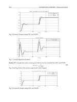
REFERENCES104
[Kailath 1980] T.Kailath. “Linear Systems”. Prentice-Hall, Englewood Cliffs,
NJ, 1980.
[Khalil 2001]. H.Khalil. “Nonlinear Systems”. Prentice-Hall, Englewood
Cliffs, NJ, 2001.
[LaSale and Lefschetz 1961] P.LaSale and S.Lefschetz. “Stability by
Lyapunov’s Direct Method”. Academic Press, New York, 1961.
[Ljung 1999] L.Ljung. “System Identification-Theory for the User”. Prentice-
Hall, Englewood Cliffs, NJ, 1999.
[Narendra and Taylor 1973] K.S.Narendra and J.H.Taylor. “Frequency
Domain Criteria for Absolute Stability”. Academic Press, New York,
1973.
[Niculescu and Abdallah 2000] S I.Niculescu and C.T.Abdallah. “Delay
Effects on Static Output Feedback Stabilization”. Submitted IEEE CDC
2000, Sydney, Australia, 2000.
[Ortega and Spong 1988] R.Ortega and M.Spong. “Adaptive Motion Control
of Rigid Robots: A Tutorial”. Proc. IEEE Conf. Dec. and Cont., pp.
1575–1584, 1988.
[Ortega et al. 1998] R.Ortega and A.Loria and P.J.Nicklasson and H.Sira-
Ramirez. “Passivity-based Control of Euler-Lagrange Systems”. Springer-
Verlag, Berlin, 1998.
[Strang 1988] G.Strang. “Linear Algebra and its Applications”. Brooks/Cole,
Stamford, CT, 1988.
[Koltchinskii et al. 1999] V.Koltchinskii and C.T.Abdallah and M.Ariola
and P.Dorato and D.Panchenko. “Statistical Learning Control of
Uncertain Systems: It is better than it seems”. IEEE Trans, on Automatic
Control, February 1999.
[Sastry and Bodson 1989] S.Sastry and M.Bodson. “Adaptive Control:
Stability, Convergence, and Robustness”. Prentice-Hall, Englewood
Cliffs, NJ, 1989.

[ATM 1996] “ATM Forum Traffic Management Specification”. ATM Forum
Traffic Management Working Group AF-TM-0056.000, version 4.0,
April 1996.
[Niculescu et al. 1997] S I.Niculescu and E.Verriest and L.Dugard and J
M.Dion. “Stability and robust stability of time-delay systems: A guided
tour”. LNCIS, Springer-Verlag, London, vol. 228, pp. 1–71, 1997.
Copyright © 2004 by Marcel Dekker, Inc.
105REFERENCES
[CDC 1999] “CDC 1999 Special session on time-delay systems”. Proc. 1999
CDC, Phoenix, AZ, 1999.
[Verhulst 1997] H.Verhulst. “Nonlinear Differential Equations and
Dynamical Systems”. Springer-Verlag, Berlin, 1997.
[Vidyasagar 1992] M.Vidyasagar. “Nonlinear Systems Analysis”. Prentice-
Hall, Englewood Cliffs, NJ, 1992.
Copyright © 2004 by Marcel Dekker, Inc.
107
Chapter 3
Robot Dynamics
This chapter provides the background required for the study of robot
manipulator control The arm dynamical equations are derived both in the
second-order differential equation formulation and several state-variable
formulations. Some important properties of the dynamics are introduced. We
show how to include the dynamics of the arm actuators, which may be electric
or hydraulic motors.
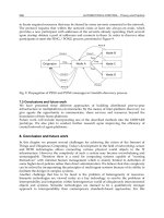
3.1 Introduction
Robotics is a complex field involving many diverse disciplines, such as physics,
properties of materials, statics and dynamics, electronics, control theory, vision,
signal processing, computer programming, and manufacturing. In this book
our main interest is control of robot manipulators. The purpose of this chapter
is to study the dynamical equations needed for the study of robot control.

For those desiring a background in control theory, Chapter 2 is provided.
For those desiring a background in the basics of robot manipulators, in Appendix
A we examine the geometric structure of robot manipulators, covering basic
manipulator configurations, kinematics, and inverse kinematics. There we
review as well the manipulator Jacobian, which is essential for control in
Cartesian or workspace coordinates, where the desired trajectories of the arm
are usually specified to begin with.
The robot dynamics are derived in Section 3.2. Lagrangian mechanics are
used in this derivation. In Section 3.3 we review some fundamental properties
of the arm dynamical equation that are essential in subsequent chapters for
which is referred to throughout the text.
The arm dynamics in Section 3.2 are in the form of a second-order vector
Copyright © 2004 by Marcel Dekker, Inc.
the derivation of robot control schemes. These are summarized in Table 3.3.1,
Robot Dynamics108
differential equation. In Section 3.4 we show several ways to convert this
formulation to a state-variable description. The state-variable description is a
first-order vector differential equation that is extremely useful for developing
many arm control schemes. Feedback linearization techniques and Hamiltonian
mechanics are used in this section.
The robot arm dynamics in Section 3.2 are given in joint-space coordinates.
In Section 3.5 we show a very general approach to obtaining the arm
dynamical description in any desired coordinates, including Cartesian or
workspace coordinates and the coordinates of a camera frame or reference.
In Section 3.6 we analyze the electrical or hydraulic actuators that perform
the work required to move the links of a robot arm. It is shown how to
incorporate dynamical models for the actuators into the arm dynamics to
provide a complete dynamical description of the arm-plus-actuator system.
This finally leaves us in a position to move on to the next chapters, where
robot manipulator control design is discussed.

3.2 Lagrange-Euler Dynamics
For control design purposes, it is necessary to have a mathematical model
that reveals the dynamical behavior of a system. Therefore, in this section we
derive the dynamical equations of motion for a robot manipulator. Our
approach is to derive the kinetic and potential energy of the manipulator and
then use Lagrange’s equations of motion.
In this section we ignore the dynamics of the electric or hydraulic motors
that drive the robot arm; actuator dynamics is covered in Section 3.6.
Force, Inertia, and Energy
Let us review some basic concepts from physics that will enable us to better
understand the arm dynamics [Marion 1965]. In this subsection we use boldface
to denote vectors and normal type to denote their magnitudes.
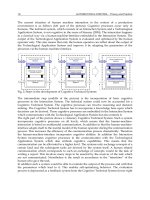
The centripetal force of a mass m orbiting a point at a radius r and angular
velocity
ω
is given by
(3.2.1)
v=w×r, (3.2.2)
which in this case means simply that v=ωr.
Copyright © 2004 by Marcel Dekker, Inc.
See Figure 3.2.1. The linear velocity is given by
Robot Dynamics110
(3.2.5)
The rotational kinetic energy of the mass in Figure 3.2.1 is given by
(3.2.6)
where the moment of inertia is
(3.2.7)
with
ρ
(r) the mass distribution at radius r in a volume. In the simple case

shown where m is a point mass, this becomes
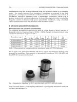
Figure 3.2.2: Coriolis force.
Copyright © 2004 by Marcel Dekker, Inc.
111
I=mr
2
. (3.2.8)
Therefore,
(3.2.9)
The potential energy of a mass m at a height h in a gravitational field with
constant g is given by
P=mgh. (3.2.10)
The origin, corresponding to zero potential energy, may be selected arbitrarily
since only differences in potential energy are meaningful in terms of physical
forces.
The momentum of a mass m moving with velocity v is given by
p=mv. (3.2.11)
The angular momentum of a mass m with respect to an origin from which
the mass has distance r is
Pang=r×p. (3.2.12)
The torque or moment of a force F with respect to the same origin is defined
to be
N=r×F. (3.2.13)
Lagrange’s Equations of Motion
Lagrange’s equation of motion for a conservative system are given by [Marion
1965]
(3.2.14)
where q is an n-vector of generalized coordinates q
i
,

␶
is an n-vector of
generalized forces
␶
i
,

and the Lagrangian is the difference between the kinetic
and potential energies
L=K-P. (3.2.15)
In our usage, q will be the joint-variable vector, consisting of joint angles
θ
i
;
(in degrees or radians) and joint offsets d
i
(in meters). Then
τ
is a vector that
has components n
i
of torque (newton-meters) corresponding to the joint
angles, and f
i
of force (newtons) corresponding to the joint offsets. Note that
we denote the scalar components of
τ
by lowercase letters.
3.2 Lagrange-Euler Dynamics
Copyright © 2004 by Marcel Dekker, Inc.

Robot Dynamics112
We shall use Lagrange’s equation to derive the general robot arm dynamics.
Let us first get a feel for what is going on by considering some examples.
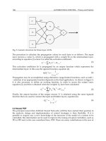
EXAMPLE 3.2–1: Dynamics of a Two-Link Polar Arm
The kinematics for a two-link planar revolute/prismatic (RP) arm are
given in Example A.2–3. To determine its dynamics examine Figure 3.2.3,
where the joint-variable and joint-velocity vectors are
(1)
The corresponding generalized force vector is
(2)
Figure 3.2.3: Two-link planar RP arm.
Copyright © 2004 by Marcel Dekker, Inc.
113
with n a torque and fa force. The torque n and force f may be provided by
either motors or hydraulic actuators. We discuss the dynamics of actuators in
Section 3.6.
To determine the arm dynamics, we must now compute the quantities
required for the Lagrange equation.
a. Kinetic and Potential Energy
The total kinetic energy due to the angular motion and the linear motion
is
(3)
and the potential energy is
(4)
b. Lagrange’s Equation
The Lagrangian is
(5)
Now we obtain
(6)
(7)

(8)
Therefore, (3.2.14) shows that the arm dynamical equations are
(9)
(10)
This is a set of coupled nonlinear differential equations which describe the
motion q(t)=[
θ
(t) r(t)]
T
given the control input torque n(t) and force f(t). We
3.2 Lagrange-Euler Dynamics
Copyright © 2004 by Marcel Dekker, Inc.
Robot Dynamics114
shall show how to determine q(t) given the control inputs n(t) and f(t) by
computer simulation in Chapter 4.
Given our discussion on forces and inertias it is easy to identify the terms
in the dynamical equations. The first terms in each equation are acceleration
terms involving masses and inertias. The second term in (9) is a Coriolis
term, while the second term in (10) is a centripetal term. The third terms are
gravity terms.
c. Manipulator Dynamics
By using vectors, the arm equations may be written in a convenient form.
Indeed, note that
(11)
We symbolize this vector equation as
(12)
Note that, indeed, the inertia matrix M(q) is a function of q (i.e., of
θ
and r),
the Coriolis/centripetal vector V(q, ) is a function of q and , and the gravity

vector G(q) is a function of q.
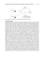
EXAMPLE 3.2–2: Dynamics of a Two-Link Planar Elbow Arm
In Example A.2–2 are given the kinematics for a two-link planar RR
arm. To determine its dynamics, examine Figure 3.2.4, where we have
assumed that the link masses are concentrated at the ends of the links.
The joint variable is
q=[
θ
1

θ
2
]
T
(1)
and the generalized force vector is
(2)
Copyright © 2004 by Marcel Dekker, Inc.
Robot Dynamics116
Therefore, the kinetic energy for link 2 is
(10)
The potential energy for link 2 is
P
2
=m
2
gy
2
=m
2

g[a
1
sin
θ
1
+a
2
sin(
θ
1
+
θ
2
)]. (11)
b. Lagrange’s Equation
The Lagrangian for the entire arm is
(12)
The terms needed for (3.2.14) are
Copyright © 2004 by Marcel Dekker, Inc.
117
Finally, according to Lagrange’s equation, the arm dynamics are given by the
two coupled nonlinear differential equations
(14)
c. Manipulator Dynamics
Writing the arm dynamics in vector form yields
(13)
3.2 Lagrange-Euler Dynamics
Copyright © 2004 by Marcel Dekker, Inc.
Robot Dynamics118
where

These manipulator dynamics are in the standard form
(17)
with M(q) the inertia matrix, V(q, ) the Coriolis/centripetal vector, and G(q)
the gravity vector. Note that M(q) is symmetric.
EXERCISE 3.2–3: Dynamics of a Three-Link Cylindrical Arm
We study the kinematics of a three-link cylindrical arm in Example A.2–
1. In Figure 3.2.5 the joint variable vector is
q=[
θ
h r]
T
(1)
Show that the manipulator dynamics are given by
(15)
(16)
Copyright © 2004 by Marcel Dekker, Inc.
Robot Dynamics120
with q the joint-variable vector and
τ
the generalized force/torque vector. In
this subsection we derive the dynamics for a general robot manipulator. They
will be of this same form.
To obtain the general robot arm dynamical equation, we determine the
arm kinetic and potential energies, then the Lagrangian, and then substitute
into Lagrange’s Equation (3.2.14) to obtain the final result [Paul 1981, Lee
et al. 1983, Asada and Slotine 1986, Spong and Vidyasagar 1989].
Arm Kinetic Energy. Given a point on link i with coordinates of
i
r with respect
to frame i attached to that link, the base coordinates of the point are

(3.2.17)
where T
i
is the 4×4 homogeneous transformation defined in Appendix A.
Note that T
i
is a function of joint variables q
1
, q
2
,…, q
i
. Consequently, the
velocity of the point in base coordinates is
(3.2.18)
Since ∂T
i
/∂q
j
=0, j>i, we may replace the upper summation limit by n, the
number of links. The 4×4 matrices ∂T
i
/∂q
j
may be computed if the arm matrices
T
i
are known.
The kinetic energy of an infinitesimal mass dm at
i

r that has a velocity of
v=[v
x
v
y
v
z
]
T
is
(3.2.19)
Thus the total kinetic energy for link i is given by

Substituting for dK
i
from (3.2.19), we may move the integral inside the
summations. Then, defining the 4×4 pseudo-inertia matrix for link i as
(3.2.20)
Copyright © 2004 by Marcel Dekker, Inc.
121
we may write the kinetic energy of link i as
(3.2.21)
Let us briefly discuss the pseudo-inertia matrix before proceeding to find the
arm total kinetic energy. Let
i
r=[x y z 1]
T

be the coordinates in frame i of the infinitesimal mass dm. Then, expanding
(3.2.20) yields

(3.2.22)
where the integrals are taken over the volume of link i. This is a constant
matrix that is evaluated once for each link. It depends on the geometry and
mass distribution of link i. In fact, in terms of the link i moments of inertia
(3.2.23)
cross-products of inertia
(3.2.24)
and first moments
3.2 Lagrange-Euler Dynamics
Copyright © 2004 by Marcel Dekker, Inc.
Robot Dynamics122
(3.2.25)
with m the total mass of link i, and
(3.2.26)
the coordinates in frame i of the center of gravity of link i, we may write
(3.2.27)
These quantities are either tabulated in the arm manufacturer’s specifications
or may be computed from quantities tabulated there.
Returning now to our development, the total arm kinetic energy may be
written as
(3.2.28)
Since the trace of a sum of matrices is the sum of the individual traces, we
may interchange summations and the trace operator to obtain

or
(3.2.29)
where the n×n arm inertia matrix M(q) has elements defined as
(3.2.30)
Copyright © 2004 by Marcel Dekker, Inc.
123

Since ∂T
i
/∂q
j
=0 for j>i, we may write this more efficiently as
(3.2.31)
Equation (3.2.29) is what we have been seeking; it provides a convenient
expression for the arm kinetic energy in terms of known quantities and the
joint variables q. Since m
jk
=m
kj
, the inertia matrix M(q) is symmetric. Since
the kinetic energy is positive, vanishing only when the generalized velocity
equal zero, the inertia matrix M(q) is also positive definite. Note that the
kinetic energy depends on q and .
Arm Potential Energy. If link i has a mass m
i
and a center of gravity
expressed in the coordinates of its frame i, the potential energy of the link is
given by
(3.2.32)
where the gravity vector is expressed in base coordinates as
(3.2.33)
If the arm is level, at sea level, and the base z-axis is directed vertically
upward, then
(3.2.34)
with units of m/s
2
.

The total arm potential energy, therefore, is
(3.2.35)
Note that P depends only on the joint variables q, not on the joint velocities
.
Noting that is the last column of the link i pseudo-inertia matrix T
i
,
we may write
(3.2.36)
with e
4
the last column of the 4×4 identity matrix (i.e., e
4
=[0 0 0 1]
T
). Lagrange’s
Equation. The arm Lagrangian is
3.2 Lagrange-Euler Dynamics
Copyright © 2004 by Marcel Dekker, Inc.
Robot Dynamics124
(3.2.37)
It is a fundamental property that the kinetic energy is a quadratic function of
the joint velocity vector and the potential energy is independent of
.
The terms required in Lagrange’s Equation (3.2.14) are now given by
(3.2.38)
(3.2.39)
(3.2.40)
Therefore, the arm dynamical equation is
(3.2.41)

Defining the Coriolis/centripetal vector
(3.2.42)
and the gravity vector
(3.2.43)
we may write
(3.2.44)
which is the final form of the robot dynamical equation we have been seeking.
The units of elements of M(q) corresponding to revolute joint variables
q
i
=θ
i
are kg-m
2
. The units of the elements of M(q) corresponding to prismatic
joint variables q
i
=d
i
are kilograms. The units of elements of V(q, )and G(q)
corresponding to revolute joint variables are kg-m
2
/s
2
. The units of elements
of V(q, ) and G(q) corresponding to prismatic joint variables are kg-m/s
2
.
Copyright © 2004 by Marcel Dekker, Inc.
125

3.3 Structure and Properties of the Robot Equation
In this section we investigate the detailed structure and properties of the
dynamical arm equations, for this structure should be reflected in the form of
the control law. The controller is simpler and more effective if the known
properties of the arm are incorporated in the design stage.
In reality, a robot arm is always affected by friction and disturbances. Therefore,
we shall generalize the arm model we have just derived by writing the
manipulator dynamics as
(3.3.1)
with q the joint variable n-vector and τ the n-vector of generalized forces.
M(q) is the inertia matrix, V(q, ) the Coriolis/centripetal vector, and G(q)
the gravity vector. We have added a friction term
(3.3.2)
with F
v
the coefficient matrix of viscous friction and F
d
a dynamic friction
term. Also added is a disturbance
τ
d,
which could represent, for instance, any
inaccurately modeled dynamics.
Friction is not an easy term to model, and indeed, may be the most contrary
term to describe in the manipulator dynamics model. Some more discussion
on friction may be found in [Schilling 1990].
We shall sometimes write the arm dynamics as
(3.3.3)
where
(3.3.4)

represents nonlinear terms.
Let us examine the structure and properties of each of the terms in the
robot dynamics equation. This study will offer us a great deal of insight
which we use in deriving robot control schemes in subsequent chapters. A
refer in the remainder of the book. As we develop each property, it will be
worthwhile to refer to Examples 3.2.1 to 3.2.3 in order to verify that the
properties indeed hold there. At the end of this section we illustrate in Example
3.3.1 several of the properties for a two-link planar elbow arm.
3.3 Structure and Properties of the Robot Equation
Copyright © 2004 by Marcel Dekker, Inc.
summary of the properties we discover is given in Table 3.3.1, to which we
127
kinetic energy is
(3.3.5)
Some expressions for M are given in the next subsection.
Another vital property of M(q) is that it is bounded above and below. That
is,
µ
1
I≤M(q)≤µ
2
I (3.3.6)
with µ
1
, and µ
2
scalars that may be computed for any given arm (see Example
3.3.1). When we say that µ
1
I≤M(q), for instance, we mean that (M(q)-µ

1
I) is
positive semidefinite. That is,
x
T
(M-µ
1
I)x≥0
for all x
ε
R
n
.
Likewise, the inverse of the inertia matrix is bounded, since
(3.3.7)
If the arm is revolute, the bounds µ
1
and µ
2
are constants, since q appears only
in M(q) through sin and cos terms, whose magnitudes are bounded by 1 (see
Examples 3.2.2 and 3.3.1). On the other hand, if the arm has prismatic joints,
then µ
1
and µ
2
may be scalar functions of q. See Example 3.2.1, where M(q) is
bounded above by µ
2
=mr

2
(if r>1).
The boundedness property of the inertia matrix may also be expressed as
m
1
≤||M(q)||≤m
2
, (3.3.8)
where any induced matrix norm can be used to define the positive scalars m
1
and m
2
.
Properties of the Coriolis/Centripetal Term
A glance at (3.2.42) reveals a problem that, if not understood, can make the
study of robot dynamics confusing. Simplification of this V(q, ) term would
require taking the derivative of a matrix [i.e., M(q)] with respect to the n-
vector q. However, such derivatives are not matrices, but tensors of order
three-that is, they must be represented by three indices, not two. There are
several ways to get around this problem, involving several definitions of
some new quantities.
3.3 Structure and Properties of the Robot Equation
Copyright © 2004 by Marcel Dekker, Inc.
Robot Dynamics128
Kronecker Product Analysis of V(q, ) Let us first examine the term V(q,
) from the point of view of the Kronecker product [Brewer 1978], defined for
two matrices as
(3.3.9)
where A has elements a
ij

and [a
ij
B] means the np×mq block matrix composed
of the p×q blocks a
ij
B. Thus, for we, have

For matrices A(q), B(q), with
, define the matrix derivative as
(3.3.10)
Then we may prove the product rule
(3.3.11)
with I
n
the n×n identity.
Now we may examine the Coriolis/centripetal vector V(q, )[Koditschek
1984, Gu and Loh 1988]. Using (3.3.11) twice on (3.2.42), we may obtain
(3.3.12)
or
(3.3.13)
where
(3.3.14)
(3.3.15)
Copyright © 2004 by Marcel Dekker, Inc.
129
with the matrix coefficient given by
(3.3.16)
To find an equivalent expression for V
m1
, note that

(3.3.17)
which may be written as
(3.3.18)
(Note that ∂M/∂q
i
is symmetric.) Therefore,
(3.3.20)
whence using appropriate definitions we may write
(3.3.21)
It is also possible to write (see the Problems)
(3.3.22)
Since V
v
( ) is linear in it follows that V(q, ) is quadratic in q. In fact, it
can be shown (see the Problems) that
or as
3.3 Structure and Properties of the Robot Equation
Copyright © 2004 by Marcel Dekker, Inc.
Robot Dynamics130
(3.3.23)
for appropriate definition of V
i
(q) [Craig 1988]. Indeed, the V
i
(q) are symmetric
n×n matrices.
Since V(q,
) is quadratic in , it can be bounded above by a quadratic
function of . That is,
(3.3.24)

with v
b
(q) a known scalar function and ||·|| any appropriate norm. For a
revolute arm, v
b
is a constant independent of q. See Examples 3.2.2 and
3.3.1, where the quadratic terms in are multiplied by sin θ
2
, whose magnitude
is bounded by 1. On the other hand, for an arm with prismatic joints v
b
(q)
may be function of q; see Examples 3.2.1 and 3.2.3, where V(q, ) has a term
in r multiplying the quadratic terms .
To assist in determining v
b
(q) for a given robot arm, note that so that
so that

where (q) is defined in (3.3.23). Therefore, for a revolute arm
(3.3.25)
We may note that
(3.3.26)
This is an n
2
-vector consisting of all possible products of the components of .
This and (3.3.19) allow us to demonstrate that
(3.3.27)
In this proof, we also need the identity
Copyright © 2004 by Marcel Dekker, Inc.

Lagrange-Euler Dynamics 131
(3.3.28)
for any matrices A and B. Note: It is not true that
Now we may use these various identities to show that
(3.3.29)
Thus
(3.3.30)
with
(3.3.31)
Note that, in general, V
m1
≠V
m2
.
In terms of M and U, the arm dynamics may be written as
(3.3.32)
At this point we may prove an identity that is extremely useful in constructing
advanced control schemes. We call it the skew-symmetric property; it shows
that the derivative of M(q) and the Coriolis vector are related in a very particular
way. In fact,
(3.3.33)
since a matrix minus its transpose is always skew symmetric. This important
identity holds also if V
m1
is used in place of V
m2
.
It is important to note that the first equality in (3.3.33) holds because
multiplies . That is, , so that it is not necessarily true
that (M-2V

m2
) itself is skew symmetric. However, it is possible to define a
matrix such that
(3.3.34)
and
Copyright © 2004 by Marcel Dekker, Inc.
Robot Dynamics132
(3.3.35)
is skew symmetric, so that x
T
Sx=0 for all x ⑀ R
n
Indeed, according to (3.3.13),
(3.3.27) we may define
(3.3.36)
for then the skew-symmetric matrix is nothing but
(3.3.37)
This V
m
is the standard one used in several modern adaptive and robust
control algorithms, and it is the definition we shall use in the remainder of the
book. Thus we shall write the arm equation either as
(3.3.38)
or
(3.3.39)
Note that it is possible to split V(q, ) into its Coriolis and centripetal
components as
(3.3.40)
where
(3.3.41)

and is (3.3.26) with all the square terms removed [Craig 1988] (see
the Problems).
Componentwise Analysis of . An alternative to the Kronecker product
analysis of the Coriolis/centripetal vector is an analysis in terms of the scalar
components of , which yields additional insight.
In terms of the components m
kj
(q) of the inertia matrix M(q) we may write
(3.2.38)–(3.2.40) componentwise as
Copyright © 2004 by Marcel Dekker, Inc.