Robot Manipulator Control Theory and Practice - Frank L.Lewis Part 11 doc

Advanced Control Techniques390
EXAMPLE 7.2–1: DCAL for the Two-Link Arm
We wish to design and simulate the DCAL given in Table 7.2.1 for the
two-link arm given in Figure 6.2.1. (The dynamics for this robot arm are
given in Chapter 3.) Assuming that the friction is negligible and the link
lengths are exactly known to be of length 1 m each, the DCAL can be
written as
(1)
and
(2)
In the expression for the control torques, the regression matrix Y
d
(·) is
given by
(3)
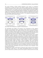
Figure 7.2.1: Block diagram of DCAL controller.
Copyright © 2004 by Marcel Dekker, Inc.
7.2 Robot Controllers with Reduced On-Line Computation 391
where
Formulating the adaptive update rule as given in Table 7.2.1, the
associated parameter estimate vector is

with the adaptive update rules
(8)
For m
1
=0.8 kg and m
2
=2.3 kg, the DCAL was simulated with

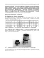
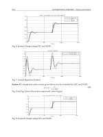
The tracking error and mass estimates are depicted in Figure 7.2.2. As
illustrated by the figure, the tracking error is asymptotically stable, and the
parameter estimates remain bounded.
(9)
and
and
Copyright © 2004 by Marcel Dekker, Inc.
7.2 Robot Controllers with Reduced On-Line Computation 393
are repeatable if the desired trajectory is periodic. That is, even though there
may be unknown constant parametric quantities in (7.2.29), the signal
represented by the n×1 vector u
d
(t) will be periodic or repeatable. Therefore,
in the subsequent discussion, we assume that the desired trajectory is periodic
with period T. This periodic assumption on the desired trajectory allows us to
write
u
d
(t)=u
d
(t-T) (7.2.30)
since the dynamics represented by u
d
(t) depend only on periodic quantities.
Utilizing the repeatability of the dynamics given by (7.2.29), the RCL is
formulated as
(7.2.31)
where the n×1 vector û
d
(t) is a learning term that is used to compensate for the

repeatable dynamics u
d
(t), and all other quantities are the same as those defined
for the DCAL. The learning term û
d
(t) is updated from trial to trial by the
learning update rule
(7.2.32)
where k
L
is a positive scalar control gain.
As done similarly in the adaptive control development, we will write the
learning update rule given in (7.2.32) in terms of the learning error, which is
defined as
(7.2.33)
Specifically, multiplying (7.2.32) by -1 and then adding u
d
(t) to both sides of
(7.2.32) yields
(7.2.34)
By utilizing the periodic assumption given by (7.2.30), we can write (7.2.34)
as
(7.2.35)
which gives the learning error update rule
(7.2.36)
where is defined in terms of (7.2.33).
Copyright © 2004 by Marcel Dekker, Inc.
Advanced Control Techniques394
Before we analyze the stability of the controller given in (7.2.31), we will
form the corresponding error system. First, we rewrite (7.2.1) in terms of r

defined in (7.2.6). That is, we have
(7.2.37)
where the n×1 vector u
a
(t) is used to represent the “actual manipulator
dynamics” given by
(7.2.38)
Adding and subtracting the term u
d
(t) on the right-hand side of (7.2.37) yields
(7.2.39)
where is defined as
(7.2.40)
As shown similarly in [Sadegh and Horowitz 1990], this difference between
the actual manipulator dynamics (i.e., u
a
(t)) and the repeatable manipulator
dynamics (i.e., u
d
(t)) can be quantified as
(7.2.41)
where ␨
1
, ␨
2
, ␨
3
, and ␨
4
are positive bounding constants that depend on the

desired trajectory and the physical properties of the specific robot configuration
(i.e., link mass, link length, friction coefficients, etc.).
The last step in forming the error system is to substitute the control given
by (7.2.31) into (7.2.39) to yield
(7.2.42)
We now analyze the stability of the error system given by (7.2.42) with the
Lyapunov-like function
(7.2.43)
Differentiating (7.2.43) with respect to time yields
Copyright © 2004 by Marcel Dekker, Inc.
7.2 Robot Controllers with Reduced On-Line Computation 395
(7.2.44)
Substituting the error system given by (7.2.42) into (7.2.44) yields
(7.2.45)
By utilizing the skew-symmetric property and the learning error update law
in (7.2.36), it is easy to show that the second line in (7.2.45) is equal to

Therefore, by invoking the definition of r given in (7.2.6), (7.2.45) simplifies
to
(7.2.46)
From (7.2.46) we can place an upper bound on in the following manner:
(7.2.47)
The rest of the stability argument is a modification of the stability argument
presented in the preceding section for the DCAL. Specifically, we first note
that (7.2.18) and (7.2.47) are almost identical since in (7.2.18) and in
(7.2.47) are bounded by the same scalar function. After one retraces the steps
of the DCAL stability argument, we can see that the controller gains k
a
and k
p

should still be adjusted according to (7.2.22) and (7.2.25), respectively.
However, the controller gain k
v
, is adjusted in conjunction with the controller
gain k
L
to satisfy
(7.2.48)
where ␨
1
, ␨
2
, ␨
3
, and ␨
4
are defined (7.2.41). If the controller gains are adjusted
according to (7.2.22), (7.2.25), and (7.2.48), then from the analytical
Copyright © 2004 by Marcel Dekker, Inc.
Advanced Control Techniques396
development given for the DCAL (i.e., (7.2.18) to (7.2.24)) and (7.2.47), we
can place the new upper bound on :
(7.2.49)
where λ
3
is a positive scalar constant given by λ
min
{Q
0
},

We now detail the type of stability for the tracking error. First note that
from (7.2.49), we can place the new upper bound on :
Multiplying (7.2.51) by -1 and integratisg the left-hand side of (7.2.51) yields
(7.2.52)
Since is negative semidefinite as delineated by (7.2.49), we can state that V
is a nonincreasing function and therefore is upper bounded by V(0). By recalling
that M(q) is lower bounded as delineated by the positive-definite property of
the inertia matrix, we can state that V given in (7.2.43) is lower bounded by
zero. Since V is nonincreasing, upper bounded by V(0), and lower bounded by
zero, we can write (7.2.52) as
(7.2.53)
or
The bound delineated by (7.2.54) informs us that (see Chapter 2),
which means that the filtered tracking error r is bounded in the “special” way
given by (7.2.54).
(7.2.50)
which implies that
(7.2.51)
(7.2.54)
Copyright © 2004 by Marcel Dekker, Inc.
7.2 Robot Controllers with Reduced On-Line Computation 397
To establish a stability result for the position tracking error e, we establish
the transfer function relationship between the position tracking error and the
filtered tracking error r. From (7.2.6), we can state that
e(s)=G(s)r(s), (7.2.55)
where s is the Laplace transform variable,
G (s)=(sI+I)
-1
, (7.2.56)

and I is the n×n identity matrix. Since G(s) is a strictly proper, asymptotically
stable transfer function and , we can use Theorem 2.4.7 in Chapter 2 to
state that
(7.2.57)
Therefore, if the controller gains are selected according to (7.2.22), (7.2.25),
and (7.2.48), the position tracking error e is asymptotically stable. In accordance
with the theoretical development presented in this section, all we can say
about the velocity tracking error e is that it is bounded. It should be noted that
if the learning estimate û
d
(t) in (7.2.32) is “artificially” kept from growing,
we can conclude that the velocity tracking error is asymptotically stable [Sadegh
et al. 1990]. The stability proof for this modification is a straightforward
application of the adaptive control proofs presented in Chapter 6.
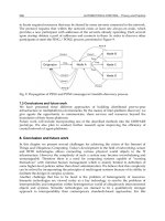
The repetitive controller examined in this section is summarized in Table
7.2.2 and depicted in Figure 7.2.3. After glancing through Table 7.2.2, we
can see that the RCL requires very little information about the robot being
controlled as opposed to adaptive controllers that required the formulation of
regression-type matrices. Another obvious advantage of the RCL is that it
requires very little on-line computation. We now present an example to illustrate
how Table 7.2.2 can be used to design repetitive controllers for robot
manipulators.
EXAMPLE 7.2–2: RCL for the Two-Link Arm
We wish to design and simulate the RCL given in Table 7.2.2 for the two-link
arm given in Figure 6.2.1. (The dynamics for this robot arm are given in
Chapter 3.) From Table 7.2.2, the RCL can be written as
(1)
and
Copyright © 2004 by Marcel Dekker, Inc.
Advanced Control Techniques400

In Chapter 5 we discussed the use of robust controllers for the control of
robot manipulators. Two of the attractive features of the robust controllers
are that on-line computation is kept to a minimum and their inherent robustness
to additive bounded disturbances. One of the disadvantages of the robust
control approach is that these controllers require a priori known bounds on
the uncertainty. In general, calculations of the bounds on the uncertainty can
be quite a tedious process since this calculation involves finding the maximum
values for the mass and friction related constants for each link of the robot
manipulator. Another disadvantage of the robust control approach is that
even in the absence of additive bounded disturbances, we cannot guarantee
asymptotic stability of the tracking error. In general, it would be desirable to
obtain at least a “theoretical” asymptotic stability result for the tracking
error.
In this section an adaptive robust controller is developed for the tracking
control of robot manipulators. The adaptive robust controller can be thought
of as combining the best qualities of the adaptive controller and the robust
controller. This control approach has the advantages of reduced online
calculations (compared to the adaptive control method), robustness to additive
bounded disturbances, no a priori knowledge of system uncertainty, and
asymptotic tracking error performance.
For purposes of control design in this section, we assume that the robotic
manipulator is a revolute manipulator with dynamics given by
(7.3.1)
where F
d
is a n×n positive definite, diagonal matrix that is used to represent
the dynamic coefficients of friction, vector containing the
Figure 7.2.4: Simulation of RCL.
Copyright © 2004 by Marcel Dekker, Inc.
7.3 Adaptive Robust Control 401

static friction terms, T
d
is a n×1 vector representing an unknown bounded
disturbance, and all other quantities are as defined in Chapter 3.
The adaptive robust controller is very similar to the robust control strategies
discussed in Chapter 5 in that an auxiliary controller is used to “bound” the
uncertainty. Recall from Chapter 5 that the robust controllers bounded the
uncertainty by using a scalar function that was composed of tracking error
norms and positive bounding constants. For example, suppose that the dynamics
given by
(7.3.2)
represent the uncertainty for a given robot controller. That is, the dynamics
given by (7.3.2) are uncertain in that payload masses, coefficients of friction,
and disturbances are not known exactly. It is assumed; however, that a positive
scalar function
ρ
can be used to bound the uncertainty as follows:
(7.3.3)
As delineated in [Dawson et al. 1990], the physical properties of the robot
manipulator can be used to show that the dynamics given by (7.3.2) can be
bounded as
(7.3.4)
and δ
0
, δ
1
, and δ
2
are positive bounding constants that are based on the largest
possible payload mass, link mass, friction coefficients, disturbances, and so on.

In general, the robust controllers presented in Chapter 5 required that the
bounding constants defined in (7.3.4) be formulated a priori. The adaptive
robust controller that will be developed in this section “learns” these bounding
constants on-line as the manipulator moves. That is, in the control
implementation, we do not require knowledge of the bounding constants;
rather, we only require the existence of the bounding constants defined in
(7.3.4).
Similar to the general development presented in [Corless and Leitmann
1983], the adaptive robust controller has the form
(7.3.6)
(7.3.5)
where
Copyright © 2004 by Marcel Dekker, Inc.
Advanced Control Techniques402
where K
v
is a n×n diagonal, positive-definite matrix, r (the filtered tracking
error) is defined as in (7.2.6), and v
R
is a n×1 vector representing an auxiliary
controller. The auxiliary controller v
R
in (7.3.6) is defined by
(7.3.7)
k
ε
is a positive scalar control constant, is a scalar function defined as
(7.3.9)
and are the dynamic estimates of the corresponding bounding
constants δ

0
, δ
1
, and δ
2
defined in (7.3.4). The bounding estimates denoted by
“ˆ” are changed on-line based on an adaptive update rule. Before giving the
update rule, we write (7.3.9) in the more convenient form
(7.3.10)
The actual bounding function
ρ
given in (7.3.3) can also be written in the
matrix form
(7.3.11)
Note the similarity between the regression matrix formulation in the adaptive
approach (see Chapter 6) and the formulation given by (7.3.10). Specifically,
the 1×3 matrix S resembles a “regression matrix,” and the 3×1 vector
resembles a “parameter estimate vector.”
The bounding estimates defined in (7.3.10) are updated on-line by the
relation
(7.3.12)
where r is defined in (7.2.6), S is defined in (7.3.10), and γ is a positive scalar
control constant. For convenience, we also note that since δ
0
, δ
1
, and δ
2
defined
in (7.3.4) are constants, (7.3.12) can be written as

where
(7.3.8)
where
where
Copyright © 2004 by Marcel Dekker, Inc.
7.3 Adaptive Robust Control 403
(7.3.13)
since we will define the difference between
␪
and as
(7.3.14)
We now turn our attention to analyzing the stability of the corresponding
error system for the controller given in (7.3.6). Substituting the controller
(7.3.6) into the robot Equation (7.3.1) gives the error system
(7.3.15)
where w is defined in (7.3.2).
We now analyze the stability of the error system given by (7.3.15) with the
Lyapunov-like function
(7.3.16)
Differentiating (7.3.16) with respect to time yields
(7.3.17)
since scalar quantities can be transposed. Substituting (7.3.13) and (7.3.15)
into (7.3.17) yields
(7.3.18)
By utilizing the skew-symmetric property, it is easy to see that the second line
in (7.3.18) is equal to zero. From (7.3.18), we can use (7.3.3) and (7.3.11) to
place an upper bound on V in the following manner:
(7.3.19)
Substituting (7.3.7), (7.3.8), (7.3.10) and (7.3.14) into (7.3.19), we obtain
(7.3.20)

which can be written as
Copyright © 2004 by Marcel Dekker, Inc.
Advanced Control Techniques404
(7.3.21)
Obtaining a common denominator for the last two terms in (7.3.21) enables
us to write (7.3.21) as
(7.3.22)
Since the sum of the last two terms in (7.3.22) is always less than zero, we can
place the new upper bound on :
(7.3.23)
We now detail the type of stability for the tracking error. First, note from
(7.3.23) that we can place the new upper bound on :
(7.3.24)
As illustrated for the RCL in the preceding section, we can use (7.3.24) to
show that all signals are bounded and that (see Chapter 2). Following
the RCL stability analysis, we can use (7.2.6) to show that the position tracking
error (e) is related to the filtered tracking error r by the transfer function
relationship
(7.3.25)
where s is the Laplace transform variable and G(s) is a strictly proper,
asymptotically stable transfer function. Therefore, we can use Theorem 2.4.7
in Chapter 2 to state that
(7.3.26)
The result above informs us that the position tracking error e is asymptotically
stable. In accordance with the theoretical development presented in this section,
we can only state that the velocity tracking error e and the bounding estimates
are bounded. It should be noted that in [Corless and Leitmann 1983], a
more complex theoretical development is presented that proves the velocity
tracking error is asymptotically stable. However, in the interest of brevity
this additional information is left for the reader to pursue.

Copyright © 2004 by Marcel Dekker, Inc.
7.3 Adaptive Robust Control 405
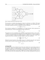
The adaptive robust controller derived in this section is summarized in
Table 7.3.1 and depicted in Figure 7.3.1. We now present an example to
illustrate how Table 7.3.1 can be used to design adaptive robust controllers
for robot manipulators.
EXAMPLE 7.3–1: Adaptive Robust Controller for the Two-Link Arm
We wish to design and simulate the adaptive robust controller given in Table
7.3.1 for the two-link arm given in Figure 6.2.1. (The dynamics for this robot
arm are given in Chapter 3.) To model friction and disturbances, the dynamics
(1)
and
Table 7.3.1: Adaptive Robust Controller
Copyright © 2004 by Marcel Dekker, Inc.
Advanced Control Techniques406
(2)
were added to respectively, in the two-link robot model.
We can now use Table 7.3.1 to formulate the adaptive robust controller as
(3)
In the expression above for the control torques, the bounding function is
given by
(5)
where From Table 7.3.1, the associated bounding
estimates are updated in the fashion
(6)
For m
1
=0.8 kg, m
2
=2.3 kg, and link lengths of 1 m each, the adaptive

robust controller was simulated with the control parameters, initial conditions,
and desired trajectory given by

and
(4)
and
Copyright © 2004 by Marcel Dekker, Inc.
Advanced Control Techniques408
in many robot control researchers’ opinions, it is now time to begin to include
the effects of actuator dynamics in the control synthesis. Recently, several
researchers have postulated that the detrimental effects of actuators are
preventing high-speed motion/force control of robot manipulators [Eppinger
and Seering 1987].
In this section we illustrate how a systematic approach can be used to
compensate for actuator dynamics in the form of electrical effects and joint
flexibilities. Using this approach and the assumption of exact model knowledge,
controllers are developed that yield a global asymptotic stability result for
the link tracking error. Although we assume exact knowledge of the model, it
is important to realize that in some cases, it may be possible to formulate
adaptive and robust nonlinear tracking controllers to compensate for
“uncertainty.” The compensation of uncertain systems in the presence of
actuator dynamics is currently being researched [Ghorbel and Spong 1990].
Electrical Dynamics
In this subsection, we illustrate how a “corrective” controller [Kokotovic et
al. 1986] can be synthesized that ensures asymptotic link tracking despite the
electrical dynamics that a motor will add to the overall system dynamics.
The terminology corrective controller is used to emphasize the fact that the
controller corrects for the electrical dynamics. The class of robots studied in
this subsection will be referred to as rigid-link electrically driven (RLED)
robots. For simplicity, we assume that the ac-tuator is a direct-current (dc)

Figure 7.3.2: Simulation of adaptive robust controller.
Copyright © 2004 by Marcel Dekker, Inc.
7.4 Compensation for Actuator Dynamics 409
motor; however, the following analysis, with some modifications, can be
used for more complicated motors such as the switched-reluctance motor
[Taylor 1989].
The model [Tarn et al. 1991] for the RLED robot is taken to be
(7.4.1)
(7.4.2)
(7.4.3)
M(q) is a n×n link inertia matrix, is a n×I vector containing the
centripetal, Coriolis, gravity, damping, and friction terms, J is a n×n constant,
diagonal, positive-definite matrix used to represent the actuator inertia, I(t) is
an n×1 vector used to denote the current in each actuator, K
T
is a constant
diagonal n×n matrix used to represent the conversion between torque and
current, L
a
is a n×n constant positive-definite diagonal matrix used to represent
the electrical inductance, is a n×1 vector used to represent the electrical
resistance and the motor back-electromotive force, and u
E
(t) is an n×1 control
vector used to represent the input motor voltage.
Throughout the book, a good deal of emphasis has been placed on the
utilization of physical properties of robot manipulators to aid us in the stability
analysis. In this tradition we note that the composite inertia matrix M(q)
defined in (7.4.3) is symmetric, positive definite, and is uniformly bounded as
a function of q; therefore, we can state for any n×1 vector x that

(7.4.4)
where m
1
is a positive scalar constant that depends on the mass properties
of the specific robot (see Chapter 3). From (7.4.4), it can also be established
that
(7.4.5)
where ||·||
i2
is used to denote the induced 2-norm (see Chapter 2).
As discussed many times before, we are interested in the performance of
the link tracking error. To avoid confusion, we restate that the tracking error
is defined to be
where
Copyright © 2004 by Marcel Dekker, Inc.
Advanced Control Techniques410
(7.4.6)
where q
d
represents the desired link trajectory. We will assume that q
d
and its
first, second, and third derivatives are all bounded as functions of time. We
also assume that the first derivative of the link dynamics on the left-hand side
of (7.4.1) exists. These assumptions on the “smoothness” of the desired trajectory
and the link dynamics ensure that the controller, which will be developed
later, remains bounded.
The control objective will be to obtain asymptotic link tracking despite the
electrical dynamics. To accomplish this objective, we first rewrite (7.4.1) in
terms of the tracking error given by (7.4.6) to yield

(7.4.7)
The error system given by (7.4.7) can also be written in the state-space form
(7.4.8)
O
n×n
is the n×n zero matrix, and I
n×n
is the n×n identity matrix.
As one can plainly see, there is no control input in (7.4.8); therefore, we
will add and subtract the term BM
-1
(q)u
L
on the right-hand side of (7.4.8) to
yield
(7.4.9)
where u
L
is an n×1 vector representing a “fictitious” n×1 control input. As it
turns out, the controller u
L
is the computed-torque controller that ensures
asymptotic link tracking error if the electrical dynamics were not present. As
we will see later, the fictitious controller u
L
is actually embedded inside the
overall control strategy, which is designed at the voltage control input u
E
.
Continuing with the error system development, we define u

L
for RLED
robots to be the computed-torque controller
(7.4.10)
where
Copyright © 2004 by Marcel Dekker, Inc.
7.4 Compensation for Actuator Dynamics 411
where K
Lv
and K
Lp
are defined to be n×n positive-definite diagonal matrices.
Substituting (7.4.10) for only the first u
L
term in (7.4.9) yields the link tracking
error system
(7.4.11)
With regard to the link tracking error system given by (7.4.11), if
η
E
could
be guaranteed to be zero for all time, we could easily show that the tracking
error would be asymptotically stable since A
L
defined in (7.4.12) has stable
eigenvalues. Therefore, one can view the control objective as forcing the
“perturbation”
η
E
to go to zero.

To design a control law for
η
E
, we must first establish its dynamic
characteristics. From (7.4.12), the derivative of
η
E
with respect to time is
given by
(7.4.13)
To obtain the the dynamic characteristics of
η
E
, we substitute for in (7.4.13)
from (7.4.2) to yield
(7.4.14)
We can now use (7.4.14) to design a control law at the input u
E
to force
η
E
to go to zero. The fact that
η
E
should go to zero motivates the corrective
control law
(7.4.15)
where K
Ep
is defined to be a n×n positive-definite diagonal matrix. Substituting

(7.4.15) into (7.4.14) yields
(7.4.16)
The dynamic equations given by (7.4.11) and (7.4.16) can be thought of as
two interconnected systems representing the overall closed-loop dynamics. As
one would expect, it would be desirable to determine the type of stability of
the overall closed-loop system. To determine the type of stability of (7.4.11)
and (7.4.16), we will utilize the Lyapunov function
where
(7.4.11)
(7.4.17)
Copyright © 2004 by Marcel Dekker, Inc.
Advanced Control Techniques412
where

If the sufficient condition given by
(7.4.18)
is satisfied, then by the Gerschgorin theorem (see Chapter 2), it is obvious that
P
L
is a positive-definite matrix, and hence V is a Lyapunov function. The
condition given by (7.4.18) simply means that the smallest velocity controller
gain should be larger than 1.
Differentiating (7.4.17) with respect to time yields
Note that if the sufficient condition given by (7.4.18) holds, it is obvious that
the matrix Q
L
is positive definite. Using the fact that Q
L
is positive definite
allows us to place an upper bound on given in (7.4.20). This upper bound

is given by
(7.4.22)
where m
l
is defined in (7.4.5).
To determine the sufficient conditions on the controller gains for asymptotic
stability, we rewrite (7.4.22) in the matrix form
(7.4.23)
where
(7.4.19)
Substituting (7.4.11) and (7.4.16) into (7.4.19) yields
where
where
Copyright © 2004 by Marcel Dekker, Inc.
7.4 Compensation for Actuator Dynamics 413
By the Gerschgorin Theorem, the matrix Q
0
defined in (7.4.23) will be positive
definite if the sufficient condition
(7.4.24)
holds. Therefore, if the controller gains satisfy the conditions given by (7.4.18)
and (7.4.24), we can use standard Lyapunov stability arguments (see Chapter
2) to state that the vector x
0
defined in (7.4.23) and hence ||e||, e, and e are all
asymptotically stable. It is easy to show that if the sufficient condition
(7.4.25)
holds, the conditions given by (7.4.18) and (7.4.24) are always satisfied.
It should be noted that the control given by (7.4.15) depends on the
measurement of u

L
, and I. At first one might be tempted to state that this
controller requires measurements of and I; however, since we have
assumed exact knowledge of the dynamic model given by (7.4.1) and (7.4.2),
we can use this information to eliminate the need for measuring q That is, by
differentiating (7.4.10) with respect to time, u
L
can be written as
(7.4.26)
After substituting for in (7.4.26), u
L
will depend only on the measurement of
q, and I. The actual control that would be implemented at the control input
u
E
can be found by making the appropriate substitution into (7.4.15). That is,
the corrective control given by (7.4.15) can be written as
(7.4.27)
where is found from (7.4.1) to be
Copyright © 2004 by Marcel Dekker, Inc.
Advanced Control Techniques414
where would be given by (7.4.26).
After examining the functional dependence of given in (7.4.26), it is
now obvious why we have assumed that the desired trajectory and the link
dynamics be sufficiently smooth. Specifically, we can see from (7.4.26) that
the corrective controller requires that the first, second, and third time derivatives
of the desired trajectory to be bounded while requiring the existence of the
first derivative of the link dynamics. These assumptions on the desired trajectory
and the link dynamics ensure that the control input will remain bounded.
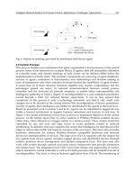
The corrective controller derived above is summarized in Table 7.4.1 and

depicted in Figure 7.4.1. We now present an example to illustrate how Table
7.4.1 can be used to design corrective controllers for RLED robots.
EXAMPLE 7.4–1: Corrective Controller for the One-Link RLED Arm
We wish to design and simulate a corrective controller using Table 7.4.1 for
the one-link motor-driven robot arm given in Figure 7.4.2. The dynamics for
the system are taken to be
(1)
where m=1kg, K
T
=2 N/A, k
b
=0.3 V-S, f
d
=3 kg-m/s, L=1 m, L
a
=0.1 H, R=5
Ω, g is the gravitational coefficient, J=0.2 kg-m
2
, I is the motor current, and u
E
is the motor input voltage.
Assuming that the model given by (1) and (2) is known exactly, we can use
Table 7.4.1 to formulate the corrective controller
(3)
and
(2)
where
(4)
Copyright © 2004 by Marcel Dekker, Inc.
7.4 Compensation for Actuator Dynamics 417

terminology corrective controller is used to emphasize the fact that the controller
corrects for the dynamics that are used to represent the effects of joint
flexibilities. The class of robots studied in this subsection will be referred to as
rigid-link flexible-joint (RLFJ) robots.
The model [Spong 1987] for the RLFJ robot is taken to be
(7.4.28)
q
m
(t) is a n×1 vector representing the motor displacement, K is a constant,
diagonal, positive-definite n×n joint flexibility matrix, is an
n×1 vector that represents the motor damping and flexibility effects, u
F
(t)
is an n×1 control vector used to represent the input torque, and all other
quantities are defined as in the preceding subsection. With regard to the
rigid link model given in (7.4.28), we note from Chapter 3 that for any
n×1 vector x
Figure 7.4.3: Simulation of RLED corrective controller.
where
(7.4.29)
(7.4.30)
Copyright © 2004 by Marcel Dekker, Inc.
Advanced Control Techniques418
(7.4.31)
where m
1
is a positive scalar constant.
As in the preceding subsection, we are interested in the performance of the
link tracking error defined in (7.4.6). For the control of RLFJ robots, we will
assume that q

d
and its first, second, third, and fourth derivatives are all bounded
as functions of time. We also assume that the first and second derivatives of
the link dynamics on the left-hand side of (7.4.28) exist. These assumptions
on the “smoothness” of the desired trajectory and the link dynamics ensure
that the controller, developed later, remains bounded.
Following the same analytical development given in the previous sections,
we write (7.4.28) in terms of the tracking error given by (7.4.6) to yield the
state-space form
(7.4.32)
where A
0
, e, and B are defined as in (7.4.8). Again, since there is no control
input in (7.4.32); we add and subtract the term BM
-1
(q)u
L
on the right-hand
side of (7.4.32) to yield
(7.4.33)
where u
L
is again used to represent a fictitious n×1 control input. As before,
the fictitious controller u
L
will be embedded inside the overall control strategy,
which is designed at the control input u
F
.
Continuing with the error system development, we define u

L
for RLFJ robots
to be the computed-torque controller
(7.4.34)
where K
Lv
and K
Lp
are defined as in (7.4.10). Substituting (7.4.34) into (7.4.33)
yields the link tracking error system
(7.4.35)
where A
L
is defined as in (7.4.12),
Copyright © 2004 by Marcel Dekker, Inc.
7.4 Compensation for Actuator Dynamics 419
(7.4.36)
The reason for defining
η
F
in terms of (u
L
-Kq
m
) and its derivative is that the
dynamics given by (7.4.29) are second-order dynamics. That is, since the
actuator dynamics are second order, we force
η
F
and its derivative (i.e.

η
.

F
, ) to
zero to ensure that the link tracking error (e) goes to zero.
To design a control law for
η
F
, we must first establish its dynamic
characteristics. From (7.4.36), the derivative of
η
F
is given by
(7.4.37)
To obtain the the dynamic characteristics of
η
F
, we substitute for q
m
in (7.4.37)
from (7.4.29) to yield
(7.4.38)
We can now use (7.4.38) to design a control law at the input u
F
to force
η
F
to go to zero. The fact that
η

F
should go to zero motivates the control law
(7.4.39)
where K
Fv
and K
Fp
are defined to be n×n positive-definite diagonal matrices.
Substituting (7.4.39) into (7.4.38) yields
(7.4.40)
The dynamic equations given by (7.4.35) and (7.4.40) can be thought of as
two interconnected systems representing the overall closed-loop dynamics.
To determine the type of stability for the closed-loop dynamics, we will utilize
the Lyapunov function
(7.4.41)
where P
L
is defined in (7.4.17) and
where
Copyright © 2004 by Marcel Dekker, Inc.