Robot Motion Planning and Control - J.P. Laumond Part 6 ppsx
Bạn đang xem bản rút gọn của tài liệu. Xem và tải ngay bản đầy đủ của tài liệu tại đây (1.25 MB, 25 trang )
Optimal Trajectories for Nonholonomic Mobile Robots 117
(I) ql;1 + or r~+~fr$ 0 < a < ~, 0 < b < ~, 0 < e <
(II)(III) Ca]CbC~ or CaCb[Ce O < a < b , O < e < b , O < b <
(IV) CaCb]CbCe O~a<b, O<_e<b, O<_b<~
(V)
C~ICbCb]C~
0<a<b,
O <_ e < b ,
0<b<~
(VI) C~lC~S~C~lCb
O_<a<~, O_<b<-~, O_<l
(VII)(VIII) C~[C~S~Cb or CbS:C~]C~ O < a < ~r , O < b < ~ , O <_ l
(IX) C~SzCb
0<a<~, 0~l, 0<b<~
(22)
However, all the path contained in this family are obtained for ul = 1 or
ul = -1, and by this, are admissible for RS. Therefore, this family constitutes
also a sufficient family for RS which contains 46 path types. This result improves
slightly the preceding statement by Reeds and Shepp of a sufficient family
containing 48 path types.
On the other hand, as Fillipov's existence theorem guarantees the existence
of optimal trajectories for the convexified problem CRS, it ensures the existence
of shortest paths with bounded curvature radius for linking any two configura-
tions of Reeds and Shepp's car. Applying PMP to Reeds and Shepp's problem
we deduce the following lemma that will be useful in the sequel.
Lemma 11. (Necessary conditions of PMP)
Optimal trajectories for RS are of two types:
-
A/Paths lying between two parallel lines D + and D- such that the straight
line segments and the points of inflection lie on the median line Do of both
lines, and the cusp points lie on D + or D At a cusp the point's orientation
is perpendicular to the common direction of the lines (see figure 3),
- B/Paths
C]Cl IC
with
length(C) < 7r
for any C.
4.3 A
geometric approach: construction
of a synthesis of optimal
paths
Symmetry
and reduction properties
In order to analyse the variation of
the car's orientation along the trajectories let us consider the variable 8 as
a real number. To a point q = (x,y,8*) in R 2 x S I correspond a set Q =
{(x,y,8) / 8 6
8*} in R 3 where 8* is the class of congruence modulus 27r.
Therefore, the search for a shortest path from q to the origin in R 2 x S 1
is equivalent to the search for a shortest path from Q to the origin in R 3.
By considering the problem in R 3 instead of R 2 x S 1 we can point out some
interesting symmetry properties. First let us consider trajectories starting from
each horizontal plane P0 = {(x,y,8),
x,y 6
R 2} C R 3.
118 P. Sou~res and J D. Boissonnat
In the plane P of the robot's motion, or in the plane P0, we denote by A0
the line of equation: y = -x cot ~ and A~ the line perpendicular to Ao passing
through 0. Given a point (M,0), we denote by M1 the point symmetric to M
with respect to O, M2 the point symmetric to M with respect to A0, and M3
the point symmetric of M1 with respect to Ao. Let T a be path from (M, 0)
to (o, 0).
Lemma 12. There exist three paths ~, T2 and T3 each isometric to T, starting
respectively from (M1,0), (M2, 0) and (M3,0) and ending at (O,0) (see figure
5).
A o
M2
Fig. 5. A path gives rise to 3 isometric ones.
Proofi (see Figure 5) 7~ is obtained from T by the symmetry with respect to O.
Proving the existence of T2 requires us to consider the construction illustrated at
figure (6): We denote by 5 the line passing through M and making an angle 8 with the
x-axis, and s the axial symmetry with respect to g. Let A be the intersecting point of
with the x-axis and r the rotation by the angle -8 around A. Let us note L = r(M).
Finally, t, represents the translation of vector LO. We denoteby 7~ the image of
T by the isometry .~ = t o r o s. 7~ links the directed point (M, 8) = -~((O, 0)) to
(O, 0) = .~(M, 8). 0 clearly equals 0. We have to prove that M = M2. Let respectively
and/~ be the angles made by (O,M) and (O,/~/) with the x-axis. The measure of
the angle made by the bisector of (M, O, ]vl) and the x-axis is: (1+ ~ = ~ = ~2 A.
As tan ~-~ = - cot ~, we can assert that ~/is the symmetric point of M with respect
to Ale, i.e. M2.
Optimal Trajectories for Nonholonomic Mobile Robots 119
Finally 73 is obtained as the image of 7" by ~ followed by the symmetry with
respect to the origin. [:]
M=M2
Fig. 6. Construction of the isometry ~.
Lemma 13. If T is a path from
(M(x,y),O)
to (O,0), there exists a path T,
isometric to T, from
(M(x,-y),-8)
to (0, 0).
Proof: It suffices to consider the symmetry s~ with respect to the abscissa axis.
Remark 7. -
By combining the symmetry with respect to Ao and the sym-
metry with respect to O, the line A~ appears to be also an axis of symmetry.
According to lemmas 12 and 13 it is enough to consider paths starting from
one quadrant in each plane Po, and only for positive or negative values of
O.
- The constructions above allow us to deduce easily the words wl, w2, w3 and
w4 describing ~, 7-2, 7-3 and 7-4 from the word w describing T.
• wl is obtained by writing w, then by permutating the superscripts +
and -
• w2 is obtained by writing w in the reverse direction, then by permutating
the superscripts + and -
• w3 is obtained by writing w in the reverse direction
• ~ is obtained by writing w, then by permutating the r and the t []
120 P. Sou~res and J D. Boissonnat
As a consequence of both lemmas above a last symmetry property holds in
the case that 0 q-zr:
Lemma 14.
If 7" is a path from (M(x, y), ~r) (resp. (M(x, y), -Tr)) to (0, 0),
there exists an isometric path T ~ from (M(x, y),-~r) (resp.
(M(x, y), lr) )
to
(o, 0).
The word w ~ describing 7 "1 is obtained by writing w in the opposite direction,
then by permutating on the one hand the r and the l, and on the other hand
the + and
Remark 8.
The points (M(x,y),Tr) and (M(x,y),-Tr) represent the same
configuration in R 2 x S 1 but are different in
R 3.
This means that the tra-
jectories 7" and T I are isometric and have the same initial and final points, but
along these trajectories the car's orientation varies with opposite direction.
Proof of lemma 14: We use the notation of lemma 12 and 13. Let
(M(x,y),1r)
be a directed point and T a trajectory from (M, zr) to (0, 0). When 0 = :klr the axis
Ao
is aligned with the x-axis. By lemma 12, there exists a trajectory 7~ = ~(T),
isometric to T, starting at
(M2(x,-y),rc)
and ending at (O,0). Then by lemma 12
there exists a trajectory ~ sx (7~), isometric to T2, starting at
("~2(x, y),-Tr)
and
ending at (O, 0). Let us call
T'
the trajectory ~, then
T' = s, o .~(T)
is isometric
to T and by combining the rules defining the words w2 and ~ we obtain the rule
characterizing ~-~ = w r (the same reasoning holds when 0 = -zr.) D
Now by using lemma 14 we are going to prove that it suffice to consider
paths starting from points (x, y, 0) when 0 E [-lr, ~r]. In the family (22) three
types of path may start with an initial orientation 0 that does not belong to
[-~r, ~r]. These types are (I) and (VII) &~ (VIII). Combining lemma 14 with the
necessary condition given by PMP we are going to refine the sufficient family
(22) by rejecting those paths along which the total angular variation is greater
than ~.
Lemma 15. In the family (22), types
(I), (VII)
and
(VIII)
may be refined as
follows:
(I)
l+lbl+
or
r+rb r+ O<a+b+e<~r
(VII) (VIII)
{
0<a<~,0<b<9, 0<d
CalC~SdCb
or
CbSdC~ICa
and
a+b<_ ~
if u2 is constant
on every arc C
Proof: Our method is as follows:
1. We consider a path T linking a point (M, 0) to the origin, such that Igl > ~r.
Optimal Trajectories for Nonholonomic Mobile Robots 121
2. We select a part of T located between two configurations (M1,01) and (M2, 02)
such that [01-021 = ~r. According to lemma 14 we replace this part by an isometric
one, along which the point's orientation rotates in the opposite direction. In this
way we construct a trajectory equivalent to 7" i.e having the same length and
linking (M, 0) to the origin.
3. We prove that this new trajectory does not verify the necessary conditions given
by PMP. As 7" is equivalent to this non optimal path we deduce that it is not
optimal.
Let us consider first a type (I) path. Due to the symmetry properties it suffices to
regard a path
l+l~l +
with a + b + e = ~r + e, (e > 0) and a > e. If we keep in place a
piece of length e and replace the final part using lemma 14, we obtain an equivalent
path
l+r[r+r~_~
which is obviously not optimal because the robot goes twice to the
same configuration.
We use the same reasoning to show that a path
C~IC~Sd
with d # 0 cannot be
optimal if a > ~. Without lost of generality we consider a path l + +l~_ s d . According
to lemma 14 we can replace the initial piece l + . l~ by the isometric one r+ r~+ .
The initial path is then equivalent to the path
r+_~r~+J[s -
which cannot be optimal
as the point of inflection do not belong to the line supporting the line segment.
Consider now a path
C~]C~SdCb
or
CbSdC~IC~
with u2 constant on the arcs.
We show that such a path cannot be optimal if
a+b
> ~. Consider a path
l+l~_Sdlb
2
with a + b = ~ + e and a > e. We keep in place a piece of length e and replace
the final part by an isometric one according to lemma 14. We obtain an equivalent
path
l+r+bS+dl+ra_ ~.
As the point of inflection does not lie on the line D0, this path
2
violates both necessary conditions A and B of PMP (see lemma 11) and therefore is
not optimal. [3
Remark 9.
In the sufficient family (22) refined by lemma
15,
the orientation
of initial points is defined in [-~r, 7r]. So, to solve the shortest path problem in
R 2 x S 1, we only have to consider paths starting from
R 2 x [-~, 7r]
in R 3.
Construction of domains For each type of path in the new sufficient family,
we want to compute the domains of all possible starting points for paths ending
at the origin. According to the symmetry properties it suffices to consider
paths starting from one of the four quadrants made by A0 and A~, in each
plane
Po,
and only for positive or negative values of 0. We have chosen to
construct domains covering the
first
quadrant (i.e. x tan 2°- < y ~ -x cot ~), for
e e
o].
As any path in the sufficient family is described by three parameters, each
domain is the image of the product of three real intervals by a continuous
mapping. It follows that such domains are connected in the configuration space.
To represent the domains, we compute their restriction to planes
Po.
As 0
is fixed, the cross section of the domain in
Po
is defined by two parameters. By
122 P. Sou~res and J D. Boissonnat
fixing one of them as the other one varies, we compute a foliation of this set.
This method allows us, on the one hand to prove that only one path starts from
each point of the corresponding domain, and on the other hand to characterize
the analytic expression of boundaries.
In order to cover the first quadrant we have selected one special path for
each of the nine different kinds of path of the sufficient family; by symmetry
all other domains may be obtained.
In the following we construct these domains, one by one, in Pe. For each
kind of path, integrating successively the differential system on the time inter-
vals during which (ul, u2) is constant, we obtain the parametric expression of
initial points. In each case we obtain the analytical expression of boundaries;
computations are tedious but quite easy (a more detailed proof is given in [33]).
We do not describe here the construction of all domains. We just give a
detailed account of the computation of the first domain, the eight other domains
are constructed exactly the same way. Figure 9 presents the covering of the first
quadrant in P_ ~, the different domains are represented.
,/
~y
r
X
Fig. 7. Path + - +
Construction of domain of path CICIC:
As we said in the introductive section,
Sussmann and Tang have shown that the study of family
CICIC
may be re-
stricted to paths types
l+l-l +
and
r+r-r +.
As we only consider values of 8 in
[-7r, 0] it suffice to study the type
l+l[l +
(figure 7). By lemma 15, a, b and e
are positive real numbers verifying: 0 < a + b + e < r.
Optimal Trajectories for Nonholonomic Mobile Robots 123
Along this trajectories the control
(ul,u2)
takes successively the values
(+1,+1),(-1,+1) and (+1,+1). By integrating the system (4) for each of
these successive constant values of ul and u2, from the initial configuration
(x, y, 8) to the final configuration (0, 0, 0) we get:
[ i-sinS + 2sin(b +e) -2sine
- cos 8 + 2 cos(b + e) - 2 cos e + 1
-a-b-e
(23)
Let us now consider that the value of 8 is fixed. The arclength parameter e
varies in [0,-8]; given a value of e, b varies in [0,-8- e]. When e is fixed as
b varies, the initial point traces an arc of the circle ~e of radius 2 centered at
Pe
(sin 8 + 2 sin e, - cos 8 - 2 cos e + 1)
One end point of this arc is the point E(sinS,-cos8 + 1) (when b = 0),
depending on the value of e the other end point (corresponding to b = -8 - e)
describes an arc of circle of radius 2 centered at the point H(- sin 8, cos 8 + 1)
and delimited by the point E (when e = -8) and its symmetric F with respect
to the origin O (when e = 0).
For different values of e the arcs of ~e make a foliation of the domain; this
ensures the existence of a unique trajectory of this type starting form every
point of the domain. Figure (8) represents this construction for two different
values of 8. The cross section of this domain appears at figure (9) with the
eight other domains making the covering of the first quadrant in P_ ~.
- As this domain is symmetric about the two axes A0 and A~, it follows
from lemma 12 that the domain of path
1-1+l -
is exactly the same one.
This point corroborates the result by Sussmann and Tang which states that
the search for an optimal path of the family
CICIC
(when 8 < 0) may be
limited to one of these two path types.
- When 8 = -~r the domain is the disc of radius 2 centered at the origin.
Following the same method the eight other domains are easily computed
(see [33]), they are represented at figure 9 in the plane P_~. The domain's
boundaries are piecewise smooth curves of simple sort: arcs of circle, line seg-
ments, arcs of conchoids of circle or arcs of cardioids.
Analysis of the construction As we know exactly the equations of the
piecewise smooth boundary curves, we can precisely describe the domains in
each plane P0. This construction insures the complete covering of the first
quadrant, and by symmetry the covering of the whole plane. All types in the
124 P. Sou~res and J D. Boissonnat
E e=O
0.25
0~5
I ¢,,
,,j
\
x
\
\
Fig. 8. Cross section of the domain of path
l+l[l +
in
1:>o,
(0 = -~ left side) and
(0 = -~ right side).
sufficient family are represented 3. Analysing the covering of the first quadrant,
we can note that almost all the domains are adjacent, describing a continuous
variation of the path shape. Nevertheless some domains overlap and others are
not wholly contained in the first quadrant. Therefore, if we consider the covering
of the whole plane (see fig 10), many intersections appear. In a region belonging
to more than one domain, several paths are defined, and finding the shortest
one will require a deeper study. At first sight, the analysis of all intersections
seems to be combinatorially complex and tedious, but we will show that some
geometric arguments may greatly simplify the problem. First, let us consider
the following remarks about the domains covering the first quadrant:
- Except for the domain
r+l+l-r -,
all domains are adjacent two-by-two (i.e.
they only have some parts of their boundary in common). Then, inside
the first quadrant we only have to study the intersection of the domain
r+l+l-r -
with the neighbouring domains.
- Some domains are not wholly contained in the first quadrant, therefore,
they may intersect domains covering other quadrants. Nevertheless, among
3 However, each domain is only defined for 0 belonging to a subset of [-~r, r]. So
in a given plane Pe only the domains corresponding to a subfamily of family (22)
refined by lemma 15 appear.
Optimal Trajectories for Nonholonomic Mobile Robots 125
t
-]-
_ _
]
lrv2S r~2r +
r+l lb r-
i
e I e •
i I t I
I i •
l+l~v2
s-r-
E t e2 .ip~. ' ,.r
l+l-1 +
Fig. 9. The various domains covering the first quadrant in P_ ~ (foliations appear in
dotted line).
126 P. Sou~res and J D. Boissonnat
I /AO
I
t I
I
Fig. 10. Overlapping of domains covering the plane P_
~_.
4
Optimal Trajectories for Nonholonomic Mobile Robots 127
the domains overlapping other quadrants, some are symmetric about A0
or A~ These domains are:
* the domains
l+l-l +
and
r+l+l-r-
symmetric about Ao,
, the domains
l+l-l +
and
1-s-l-
symmetric about A~, (i.e. all domains
intersecting A~ )
In this case, we consider that only one half of the domain belongs to the
covering of first quadrant. Therefore, no intersections may occur with the
symmetric domains.
Finally, we only have to study two kinds of intersections: on the one hand
the intersections of pairs of symmetric domains with respect to A0, (section
4.3), and on the other hand the intersections inside the first quadrant between
the domain
r+l+bl~r -
and the neighbouring domains (section 4.3).
Refinement of domains intersecting Ao In this section we prove that the
path
l+l-r -, l+Ibrbr+, l+l~s-r~r +,
and
l+lTs r
stop being optimal as
soon as their projections in Pe cross the Ae-axis. This will allow us to remove
the part of these domains lying out of the first quadrant.
1/Path
l+ l-r -
Lemma 16. A path
l+l-r -
linking a directed point (M(x, y), 0) to (0, 0, 0),
with y > -x cot ~, is never optimal.
Proof:
Suppose that there is a path 7~ of type
l+l-r -
from a directed point
(M1(xl,yl),81)
to (0,0,0), verifying yl > -xlcot~. Let /1//2 be the cusp point
(Figure 11). M2 is such that 4 ys < -x2cot ~. Let us consider a directed point
(M,0) moving along the path from (M1,81) to (Ms,02). As M moves, the direction
8 increases continuously from 01 to 0s. As a result, the corresponding line Ao varies
from A01 to A0:. Its slope increases continuously from cot ~ to cot ~. Then,
by continuity, there exists a directed point (M~,a) on the arc (M1, Ms), verifying
y~ = -x~ cot 8" From lemma 12, there exist two isometric paths of type
l+l-r -
and
r+l+l - linking (M~,a) to the origin. Thus, (M1,81) is linked to the origin by a path
of type
l+r+l+l -
having the same length as 7i. Such a path violates both necessary
conditions A and B of PMP (lemma 11): (A: Do and D + cannot be parallel) and
(B: us is not constant). As a consequence, 7~ is not optimal.
2/Path
l+lTs r
4 This assertion can be easily deduced from the construction of the domain of path
l-s r .
128 P. Sou~res and J D. Boissonnat
Y /Ae2 /,As A01
0 ".,',
x
Fig. 11. There exists a point M~ such that M~ E Am.
The shape of this path is close to the shape of the path
l+Ibr [ ( b = ~
and
a line segment is inserted between the last two arcs). Then, we can use exactly
the same reasoning to prove the following lemma:
Lemma 17. A path
I+lZsr -
linking a directed point
(M(x,y),O)
to (0, 0,0),
2
with y > -x cot ~, is never optimal.
3/ Path
l+lbrbr+
Lemma 18. A path
t+lbrbr+
linking a directed point
(M(x, y), 8)
to (0, 0, 0),
with y > -xcot ~, is never optimal.
Proof- The reasoning is the same as in the proof of lemma 16. Assume that there
is a path 71 of type
l+Ibrbr +
linking a directed point
(Ml(xl, yl), 81),
verifying yl >
-xl cot 9, to (0,0,0). Let M2 be the cusp-point; the subpath of 7~ from (M2,01)
to the origin is of the type
l-r-r +
symmetric to the type treated in Lemma 16.
Therefore, the coordinates of M2 must verify y2 < -x2 cot s2~. Now, let us consider a
directed point (M, 8) moving along the arc from (M1, 81) to (M2, 8). With the same
arguments as in the proof of Lemma 16, there exists a directed point (Ma, a) on this
arc, with 8t _<: a _< 82, verifying ya -x~ cot ~. From lemma 12, there exist two
isometric paths of types
l+l[rb r+
and
r-r+l+l -
linking (Ma, a) to the origin. As a
Optimal Trajectories for Nonholonomic Mobile Robots 129
result, (M1,01) is linked to the origin by a path of the type
l+r-r+l+l -
having the
same length as 7]. This path is not optimal because the robot goes twice through the
same configuration; therefore 7] cannot be optimal. []
4/Path
l+lT_s-rT_r +
2 2
The shape of this path is close to the shape of the path
l+lbrbr+ ( b - "
and a line segment is inserted between the two middle arcs). Then, we can use
exactly the same arguments to prove the next lemma.
Lemma 19. A path
l+lTs-rTr +
linking a directed point
(M(x,y),O)
to
2 2
(0,0,0), with y > -xcot ~, is never optimal.
Now, with lemmas 16 to 19 we can remove the part of domains
l+l-r -,
l+tT_s-r -, t+l-r-r +
and
l+lTs-rTr +
lying out of the first quadrant (on the
2 2 2
other side of A0). Moreover, according to the analyse made at section 4.3, we
only have to consider, the half part of the domains symmetric about A9 or A~
located in the first quadrant. As every domain intersecting A~ is symmetric
about this axis, we can construct the covering of all other quadrants with-
out generating new intersections. Inside each quadrant, it remains to study
the intersection between the domain of path
CICbCb]C
and the neighbouring
domains. Once again we restrict ourselves to the first quadrant.
Intersections inside the first quadrant
From the construction of domains
covering the first quadrant, it appears that the domain
r+l+lb r-
may intersect
the following three adjacent domains:/+/~r~r +,
l+lTs-rTr +
and
l+lTs r .
Furthermore the intersection between the domain r+l+lb r- and the domains
l+lTs-rTr +
and
l+lTs r
only happens when b is strictly greater than "
2 2 2
First, as a corollary of lemma 16, we are going to prove that a path
r+l+l[r -
is never optimal when b > ~. Therefore the corresponding part of this domain
will be removed and the intersections of domains inside the first quadrant will
be reduced to the overlapping of domains
r+l+lb r-
and
l+l~,r~r +.
Corollary 1. A path of the family
CCb[CbC
verifying b > ~ cannot be opti-
mal.
Proof: Let us consider a path of the type
r+l+lbr[.
If this path is optimal, then
the subpath
l+Ibr~
is also optimal. Integrating the corresponding system we obtain
the expression of initial points coordinates:
x = sin 0 - 2 sin(e - b) + 2 sin e
y = - cos 0 + 2 cos(e - b) - 2 cos e + 1
130 P. Sou~res and J D. Boissonnat
with ~ = e - 2b (since the first two arcs of circles have the same length) and from
lemma 16 the coordinates must verify y _< -cot ~x. Replacing x and y by their
parametric expression, we obtain after computation:
~T
e 7r (since 0<e< ~) []
sin~(2cosb-1)>0 then b< ~
Therefore according to the previous construction we may remove the part,
of the domain
r+l+l[r -
located beyond the point H with respect to O. (see
figure 9).
Now, only one intersection remains inside the first quadrant, between the
+- - +.
domains
r+l+lbr[
and
la, lb, rvre,,
let us call Z this region. In order to deter-
mine which paths are optimal in this region, we compute in each plane
Po
the
set of points that may be linked to the origin by a path of each kind having
the same length. Initial point of these two paths are respectively defined by the
following parametric systems:
(r+l+l[r:) { Y =
-sinO+ 2(2 cosb - 1) sin(e - b)
cos0 - 2(2 cosb - 1)cos(e - b) + 1
+ _ _ + {x=sin~-4sine t+2sin(e ~+b l) (2a)
(la'lb'rb're') y =
COS~ + 4COSd 2 cos(e I + b r) - 1
the length of these paths are respectively:
L = a+ 2b÷ e = 4b+ 6 with ~ = e- 2b+a
(25)
L t = e I + 2b I +a t = 2(b t +e I )-8 with 8 = e I- d
The required condition L = L ~ implies that ~ + 2b- b r - e t = 0. By replacing
e I + b ~ by ~ + 2b in the second system, then writing that both systems are
equivalent we obtain:
siu(e - b)(1 - 2 cos b) +sinO - 2sine r + sin(~ + 2b) = 0
cos(e - b)(1 2 cos b) + cos ~ - 2 cos e r +cos(O + 2b) + 1 = 0
we eliminate the parameter d writing that sin 2 (d) + cos 2 (d) = 1; then after
computation, we obtain the following relation between e and b:
4cos 2 b - 2cosb ÷ (1 - 2 cos b)(2 cos(e - 2b - 8) cosb
+ cos(e - b)) + cos ~ + cos(~ + 2b) - 1 = 0 (26)
Optimal Trajectories for Nonholonomic Mobile Robots 131
As e - 25 - 0 = e - b - (b + 0), this equation may be rewritten as follows:
A sin(e - b) + B cos(e - b) + C = 0
where A, B and C are functions of b and 0 defined by:
A = 2(1 - 2 cos b) sin(b + 8) cos b
B (1 - 2 cos 5)(2 cos(b + 0) cos b ÷ 1)
C = 4 cos 2 b - 2 cos b + cos 0 + cos(~ + 2b) - 1
Therefore we can express sin(e - b) and cos(e - b) by solving a second degree
equation; we obtain:
-AC d: tBI~/A2 + B 2 - C 2
sin(e - b) = A2 + B2
The discriminant D = A 2 ÷ B 2 - C 2 may be factored as follows:
(27)
7) = 4 cos(b) sin2(:-~)(cos(2b + 0) + cos(0) ÷ 6 cos(b) - 4)
therefore, as b E [0, ~], the sign of 7) is equal to the sign of
E(b) = cos(2b + 0) + cos(0) + 6 cos(b) - 4
Let us call bmax the value of b solution of E(b) = O. As E(b) is a decreasing
function of b, E(b) is positive when b < bmax. We will see later that the maximal
value of b we have to consider verifies this condition, ensuring our problem to
be well defined.
Now, as the region 1: is delimited by the vertical line (P2, N3), each point
belonging to 2: must verify: x < sin 0. Moreover, as the type r+l+Ib r- is defined
for b E [-0, §], we can deduce from the first line of system (24) that sin(e - b)
is negative. As a result, the choice of the positive value of the discriminant in
(27) cannot be a solution of our problem. From this condition we determine a
unique expression for sin(e - b) and cos(e - b). Replacing these expressions in
system (24) we obtain the parametric equation of a curve ~/0 issued from P2
(when b = -0), dividing the region Z into two subdomains, and crossing the
axis A0 at a point T (see figure 12). The value bT of b corresponding to the
point T may be characterized in the following manner:
From lemma 12 we know that any path of type r+l +I-~- starting on A0
a b ~b "e
verifies a e; it follows that e - b - ~ = 0. Replacing e - b by ~ in (26) bT
appears as being the solution of the implicit relation R(b) = 0, where:
132 P. Sou~res and J D. Boissonnat
0 0
R(b) = 4 cos 2 b - 2 cos b + (1 - 2 cos b)(2 cos(b + 5) cos b + cos 5) +
cos0 + cos(0 + 2b) - 1 (28)
Now, combining the relation
R(bT) = 0
with the expression of
E(bT)
we
can prove simply that
bT <bmax
in order to insure the sense of our result.
Therefore, R(b) being a decreasing function of b, the values of b e [-8,
bT]
are
the values of b e [-8, ~] verifying
R(b) >_ O.
The curve 7a is the only set of
points in I where both paths have the same length. As the distance induced
by the shortest path is a continuous function of the state, this curve is the real
limit of optimality between these two domains. This last construction achieves
the partition of the first quadrant, and by the way the partition of the whole
plane.
A 0
Q
#
/
I f
/ l
1 + 1-~-~-
HI' ~ 1 lb,~tb,l
~T ~ intersection I
/
,,=/ ~r÷l;lgr -
t I
Fig. 12. The curve 7a splitting the intersection of domains
r+l+i[r -
and
l+l~,r~,r -
in the first quadrant of P_
Description of the partition Figures (13),(14) and (15) show the partition of
the plane P0 for several values of 0 all these pictures have been traced from the
Optimal Trajectories for Nonholonomic Mobile Robots 133
4.IJ
(~-,~ :.q J ).
44 - ~
r~,, + 1_ I ,-,'~.
(~,',,,-,
~ r'7.,, t
"-~.,.;,~ ~,)
0=0
+ ,'<J:~l:l/iz, t,~,-I .
-~ "" Z-d 'T~L ~ J.'Jx ,.: ,-+ )
,~x. 71"7;/'"F,,/Az+x.',-'l
, ~ %~_~K ~2r >
(.~-x~,,,:, yf t-A ~,+;:, Qi,~')
~'s+t • L,,_++~,Jz;.~
~-;z
l.¢,x,~s r ""- Ii
$
Fig. 13. Partitions of planes Po and P_
134 P. Sou~res and J D. Boissonnat
\ ~'~' I "t /
~,,j, \
I ~4~ ~r~i<-,t,'>
• ~ L<i.,q,tf'././-k / ~ ~: £; ¢'-')
( x,'J: J,~:,,- J,'z+~,-~,._
xl** VY;I'zA
_ /, ,,~ .,+,.
~,
,.;.,
NZ,2+.~.'r",#/ t 1
\
4
i/
1'~k~+'//
Z's'±-
4.
Fig. 14. Partitions of planes P_
~-4 and P_
Optimal Trajectories for Nonholonomic Mobile Robots 135
S'r"
3~r
n
. =
4
0"0+¢ ~ /)4"
p-S" 1'~ r +
A
.,h .l. .I.,
*I.
or
. ~" 1"
.Z~I~ ~
'
Of ¢~r~
S-r-
",. +
r+~;+- r;
,
01' ~*
1+£+~z
0=-+~
Fig.
15. Partitions of
planes P_ m and P~
4
136 P. Sou~res and J D. Boissonnat
analytical equations of boundaries by using the symbolic computation software
Mathematica.
Each elementary cell consists of directed points that may be
linked to the origin by the same kind of optimal path. The 46 domains never
appear together in a plane
Po;
the following table presents the values of 0 for
which each domain exists 5
Type
cc,,IC,,C
ctc.c.lc
Intervals o] validity
[-~ ~ 0] and 'z~
, [O,,,T]
and P,d
CtC~SC
and
CSC~ tC
if
sign(u2)
is constant
CiCC
and
CCiC
CIC]SC
and
CSC~IC
[-~r,0] and [0,r]
if
sign(u2)
changes
71"
[-~r,-~] and [y, ]
ClClC
CSC
if
sign(u2 )
changes
' o] and [0,.]
CSC
[-~r, 0] and [0, ~r]
if
sign(u2)
is constant
CIC ~ SC~ IV
[-2 arccot(2), 2 arccot(2)]
When 0 varies in [-Tr, ~] the partition of planes P0 induces a partition of
R 2 x [-r, ~r]. Identifying the planes P_~ and P, we obtain a partition of the
configuration space R 2 x S 1.
In most part of domains the optimal solution is uniquely determined. How-
ever, there exist some regions of the space where several equivalent path are
defined. To describe these regions we introduce the following notation.
In the first quadrant of each plane P0, we denote by A T the half-line defined
as the part of A0 located beyond the point T (with respect to O). According to
lemmas 16 to 19, paths
l+l-r -, l+lTs-r -, t+l-~rbr +,
and
l+l~s-rTr +
stop
being optimal as soon as they cross AT, but are still optimal on A T. As the
same reasoning holds for the domains symmetric with respect to
Ao,
there exist
two equivalent paths optimal for linking any point of A T to the origin. The
same phenomenon occurs on the curve T0 where paths
r+l+blb r-
and
l+l~rb r+
have the same length. Hence, in the first quadrant, two equivalent paths are
defined at each point of A T U 70. By symmetry with respect to A0 and A~, we
can define such a set inside the four other quadrants. Let us call
No
the union
of these four symmetric sets.
5 These values of 0 have been deduced from the bounds on the parameters given by
the partition. Details are given in [34].
Optimal Trajectories for Nonholonomic Mobile Robots 137
At any point of
Po \ No = {p E Po, P ~. No}
a unique path is defined if
0 ~ zc mod(2zc).
Inside each domain the uniqueness is proven by the existence of
a foliation, and on the boundaries (outside No) any path is defined as a contin-
uous transition between two types (and belongs to both path types). However,
according to lemma 14, when ~ - 7r
mod(21r),
two equivalent (isometric) paths
are defined at any point of
Po
\ No and therefore, four equivalent paths are
defined at any point of
No.
As we have seen in the construction, there always
exist two equivalent paths (
l+l-l +
and
l-l+l -
when 0 > 0) and (r+r-r + and
r-r+r - when 0 < 0) linking any point of the central domain
C[C[C
to the
origin. Furthermore, when the initial orientation 9 equals +r, there exist two
equivalent strategies for linking any point of the plane to the origin, each one
corresponding to a different direction of rotation of the point (see lemma 14).
In that case each of the four paths
CICIC
is optimal in the central disc of
radius 2.
By choosing one particular solution in each region where several optimal
path are defined, one can determine a synthesis of optimal paths according to
definition 7. Therefore, the determination of such a synthesis is not unique.
In each cross section
Po,
the synthesis provides a complete analytic de-
scription of the boundary of domains which appear to be of simple sort: line
segment, arc of circle, arc of cardioid of circle, etc. Therefore, to characterize an
optimal control law for steering a point to the origin, it suffice to determine in
which cell the point is located, without having to do further test. This provides
a complete solution to Reeds and Shepp's problem.
On the other hand, this study constitutes an interesting way to focus on the
insufficiency of a local method, such as Pontriagyn's maximum principle, for
solving this kind of problem. The A0 axis appeared as a boundary and we had
to remove the piece of domains lying on one side of this axis. More precisely,
we have shown that any trajectory stops being optimal as it crosses the set
No. This phenomenon is due to the existence of several wavefronts intersecting
each other on this set. For this reason two equivalent paths are defined at each
point of No. (each of them corresponds to a different wave front). PMP is a
local reasoning based on the comparison of each trajectory with the trajectories
obtained by infinitesimally perturbating the control law at each time. As this
reasoning cannot be of some help to compare trajectories belonging to different
wave fronts, it is necessary to use a geometric method to conclude the study, as
we did in section 4.3 and 4.3. The main problem remains to determine
a priori
the locus of points where different wave fronts intersect.
The construction we have done for determining a partition of the phase
space required a complex geometric reasoning. In the following section we will
show how Boltianskii's verification theorem can be applied
a posteriori
to pro-
vide a simple new proof of this result.
138 P. Sou~res and J D. Boissonnat
4.4 An example of regular synthesis
In this section, we prove that the previous partition effects a regular synthesis in
any open neighbourhood of O in R 2 × S 1. First of all, we need to prove that the
curves and surfaces making up the partition define piecewise smooth sets. From
the previous construction we know that the restriction of any domain to planes
Po
is a connected region delimited by a piecewise smooth boundary curve.
Except for the curve T0 (computed at section 4.3) each smooth component
Ci(0) of the boundary remains a part of a same geometric figure Y (line, circle,
conchoid of circle, ) as 0 varies. Let Mi(0) and Ni(0) be the extremities of
the curve C~(0). As 0 varies, the position and orientation of Y" as well as the
coordinates of M~(0) and Ni(8) vary as smooth functions of 0. Therefore, in
R 2 × [-Tr, ~r], the lines trace smooth ruled surfaces, and the circles and conchoids
draw smooth surfaces. In each case we have verified that the boundary curves
Mi(0) and Ni(0) of these surfaces never connect tangentially, making sure that
all these surfaces are non singular 2-dimensional smooth surfaces.
The study of the surface T', made up by the union of the horizontal curves
"~0 when 0 varies in [-~, -~] requires more attention. As ?'0 is the region of P0
where paths r+l+'-a "b ~b re- and
l+lbrbr+
have the same length, the surface/" is
defined as the image of the set Dr = {(0,b) e R2,0 E [-~,0],b E
[-O, bT]}
by
the following mapping:
x - sin 0 + 2(2 cos b - 1) sin(e - b)
y = cos0 - 2(2 cosb - 1) cos(e - b) 4- 1
O e-2b+a
where sin(e - b) and cos(e - b) are deduced from formula (27) and
bT
is the
solution of the implicit equation
R(b)
= 0 where
R(b)
is given by (28).
Using the symbolic computation software
Mathematica
we have checked
that the matrix of partial derivatives has full rank 2 at each point of Dr.
Therefore, as the domain Dr is a 2-dimensional region of the plane (8, b) with-
out singularities, delimited by two smooth curves, F constitutes a 2-dimensional
smooth surface (see figure 16).
All the pieces of surfaces, making up the partition are 2-dimensional smooth
surfaces and from remark 4 we know that they constitute 2-dimensional piecewi-
se-smooth sets. If p2 is the union of these surfaces, p1 the union of their smooth
boundary curves Mi(O) and Ni(0), po the target point O, then in any open
neighbourhood 1) of O we can write the required relation: p0 C p1 C p2 C 1).
In order to check the regularity conditions we have considered each trajec-
tory one-by-one, following the representative point from the initial point to the
origin we have analysed the different cells encountered. We have checked that
the cell's dimension varies according to the hypothesis B of definition 9. In each
Optimal Trajectories for Nonholonomic Mobile Robots 139
0
.2 I 0
8
-i -0.6
-o12 o
Fig. 16. Set Dr (left) and surface/' (right)
case we have verified that the point never reaches the next cell tangentially. For
each trajectory we can represent this study within a table by describing from
the top to the bottom the cells ai successively crossed. Each cell corresponds
to a subpath type represented by a subword of the initial word. In each case
we specify the dimension and the type (T1) or (T2) of the cells encountered.
When the point passes from a cell ai to a cell
H(ai) = ai+l
we verify that the
trajectory riches
ai+l
with a nonzero angle ai. This is done by comparing the
vector vi tangent to the trajectory with a vector ni+l normal to
ai+l
(if ai+l is
a 2-dim cell), or with a vector wi+l tangent to
ai+l
(if ai+l is a 1-dim celt). In
any case the last cell, described in the bottom of the table, is a 1-dimensional
cell which is a piece of trajectory linking the point to Po.
Due to the lack of place we just present here the table corresponding to
paths
l+17 s-~rTr +,
an exhaustive description of all path types may be found
in [35].
140 P. Sou~res and J D. Boissonnat
Path
l+i~_s~r~re +
2 2
ceil Dim Type v~ n~ or o~
/cosek
0"1 :l+al~Sdrire+ 3 T1
Vltsi~0 )
/cosek
t3+ /
[-cose
1 /
/-cose k
/r sin6
,,4: ~,~r:_,¢ 2 T~ n,~ [-cose /
2 \2+d]
/cos8
-
2 sin ~
as : r~r+2 1T2 os tsinO+2cosO )
/-cos6~
a7 : r + 1 T1
angle t~i
n2.vl
=d+4~0
because d ) 0
then c~2 ~ 0
n4.v3=2+d¢O
because d :> 0
then a4 ~ 0
v4 and o5
not colinear
then a5 ¢ 0
/cos e~ v~ and o7
oTtsin_/)
not colinear
then (~7 ~ 0
Now, let us analyse carefully the other regularity conditions: Let N be the
set defined by N = tA0e[_~,~]Ne where No is the set defined at section 4.3
as the union of 7e, A T and their image by the axial symmetries with respect
to A6 and A~. From the previous reasoning we know that N is a piecewise
smooth set. Let v be the function defined in 1;, taking its values in the control
set U = {(ul,u2), lull = 1,and u2 E [-1, 1]} which defines an optimal control
law at each point. In each cell where more than one optimal solution exists the
choice of a constant control has been done in order to define the function v in
a unique way.
A - As stated in the beginning of this section, all the /-dim cells are i-
dimensional smooth manifolds. Moreover, as each cell corresponds to a
same path type, the control function v takes a constant value at each point
of the cell. Therefore, v is obviously continuously differentiable inside each
cell, and may be prolonged into an other constant function when the point
reaches the next cell.
B - All the 3-dim cells are of type TI
Optimal Trajectories for Nonholonomic Mobile Robots 141
-
When the representative point passes from a cell to another it never arrives
tangentially. Furthermore, as ul = 1, the velocity never vanishes.
- Along the trajectory, the variation of cell types (T1) or (T2) follows the
rule stated by Boltianskii.
C - Along any trajectory, the representative point pierces at most three cells
of type T2 and reaches the point O after a finite time.
D - From every point of N there start two trajectories having the same length
and from any point of ]) \ N there issues a unique trajectory.
E - All these trajectories satisfy the necessary conditions of PMP.
F - By crossing a border (except the set N) from a domain to another, either
the length of one elementary piece making up the trajectory vanishes, or a
new piece appears. When the point crosses the set N, the optimal strategy
switches suddenly for an isometric trajectory. Therefore, in any case, the
path length is a continuous function of the state in ]) (see [26] for more
details).
With this conditions the function v and the sets Pi effect a regular synthesis
in ];. As the point moves with a constant velocity, it is equivalent to minimize
the path length or the time, we have
f°(x,u)
- 1. Finally, as the coordinate
functions fl (x, u) =
cos ~Ul,
f2 (X, U) = sin 8Ul and f3 (x, u) = u2 have contin-
uous partial derivatives in x and u, the hypotheses of theorem 6 are verified
providing a new proof of our preceding result.
To our knowledge, this construction constitutes the first example of a regular
synthesis for a nonholonomic system in a 3-dimensional space.
5 Shortest paths for Dubins' Car
Let us now present more succinctly the construction of a synthesis of optimal
paths for Dubins' problem (DU). This results is the fruit of a collaboration
between the project
Prisme
of INRIA Sophia Antipolis and the group
Robotics
and Artificial Intelligence
of LAAS-CNRS see [10] for more details.
At first sight, this problem might appear as a subproblem of RS. Neverthe-
less, the lack of symmetry of the system, due to the impossibility for the car to
move backwards, induces strong new difficulties. Nevertheless, the method we
use for solving this problem is very close to the one developed in the preceding
section.
The work is based on the sufficient family of trajectories determined by
Dubins (14). Note that this sufficient family can also be derived from PMP
(see [36]). The study is organized as before. First, we determine the symmetry
properties of the system and we use them to reduce the state space and to refine
Dubins' sufficient family. Then, in a second time we construct the domains