Robot Motion Planning and Control - J.P. Laumond Part 9 pdf
Bạn đang xem bản rút gọn của tài liệu. Xem và tải ngay bản đầy đủ của tài liệu tại đây (1.16 MB, 25 trang )
192 A. De Luca, G. Oriolo and C. Samson
where we dropped the dependence on a for compactness.
The derivation of the reference inputs that generate a desired cartesian
trajectory of the car-like robot can also be performed for the (2, 4) chained
form. In fact, with the reference system given by
Xdl ~ ~tdl
Xd2 : Ud2
Xd3 "~" Xd2Udl
:Bd4 : Xd3ltdl,
(26)
from the output trajectory (16) and the change of coordinates (8) we easily
obtain
x~l(t) = xd(t)
x~2 (t) = [/Jd (t)~d (t) - Yd(t)~d (t)]/~] (t)
Xd3(t) = ~ld(t)/xd(t)
Xd4(t) = yd(t),
and
~dl(t) = xd(t)
Ud2(t)
= [y'd(t)x2(t)
xd(t)yd(t)xd(t) - 3~d(t)~d(t)Xd(t) + 3!]d(t)X2d(t)] /x4(t).
To work out an example for this case, consider a sinusoidal trajectory
stretching along the x axis and starting from the origin at time to = 0
Xd(t) = t, yd(t) = Asinwt.
(27)
The feedforward commands for the chained-form representation are given by
Udl(t) = 1, Ud2(t) = -Aw3 coswt,
while its initial state should be set at
Xdt(O)
=0,
Xd~(O) = O, xd3(O) =Aw, Xd4(O) =0.
We note that, if the change of coordinates (8) is used, there is an 'asym-
metric' singularity in the state and input trajectory when &d(t-) = 0, for some
> to. This coincides with the situation 8d(t-') = ~r/2, where the chained-form
transformation is not defined.
On the other hand, if the chained form comes from the model in path vari-
ables (14) through the change of coordinates (15), the state and input trajectory
needed to track the reference output trajectory
s
= sd(t),
d
= dd(t) -~
O, t >
to,
Feedback Control of a Nonholonomic Car-Like Robot 193
are simply obtained as
and
Xdl(t) : Sd(t)
Xd2(t) = 0
Xd3(t) -~ 0
Xd4(t) = 0
Udl (t) = Sd(t)
Ud2(t) = O,
without any singularity.
Similar developments can be repeated more in general, e.g., for the case of
a nonholonomic mobile robot with N trailers. In fact, once the position of the
last trailer is taken as the system output, it is possible to compute the evolution
of the remaining state variables as well as of the system inputs as functions of
the output trajectory (i.e., of the output and its derivatives up to a certain
order). Not surprisingly, the same is true for the chained form (7) by defining
(xl, x,~) as system outputs.
The above property has been also referred to as
differential flatness
[36],
and is mathematically equivalent to the existence of a dynamic state feedback
transformation that puts the system into a linear and decoupled form consisting
of input-output chains of integrators. The algorithmic implementation of the
latter idea will be shown in Sect. 3.3.
3.2 Control via approximate linearization
We now present a feedback controller for trajectory tracking based on standard
linear control theory. The design makes use of the approximate linearization of
the system equations about the desired trajectory, a procedure that leads to a
time-varying system as seen in Sect. 2.2. A remarkable feature of this approach
in the present case is the possibility of assigning a time-invariant eigenstructure
to the closed-loop error dynamics.
In order to have a systematic procedure that can be easily extended to
higher-dimensional wheeled robots (i.e., n > 4), the method is illustrated for
the chained form case. However, similar design steps for a mobile robot in
original coordinates can be found in [42].
For the chained-form representation (10), denote the desired state and input
trajectory computed in correspondence to the reference cartesian trajectory
as in Sect. 3.1 by (Xdl (t), Xd2 (t), Xd3 (t),
Xd4(t))
and
ud(t) : (Udl (t), Ud2(t))
.
Denote the state and input errors respectively as
~i=Xd~ xi, i=1, ,4, fij=u@ uj, j=l,2.
194 A. De Luca, G. Oriolo and C. Samson
The nonlinear error equations are
Xl ?~1
5
X2 = U2
X 3 = Xd2~dl
X2U 1
X 4 ~ Xd3Udl
X3~t 1.
Linearizing about the desired trajectory yields the following linear time-varying
[ 00
= 0 0
x = udl(t) 0
0 Udl(t)
system
2+
0
xd2(t) ~ = A(t)2 + B(t)~t.
d3(t)
This system shares the same controllability properties of eq. (6), which was
obtained by linearizing the original robot equations (5) about the desired tra-
jectory. For example, it is easily verified that the controllability rank condition
is satisfied along a linear trajectory with constant velocity, which is obtained
for
Ud1(t) =
Udl (a
constant nonzero value) and
Ud2(t) -~
0,
implying
Xd2(t) 0
and
Xda(t) = Xd3(to).
Define the feedback term fi as the following linear time-varying law
~1 ~
klXl (28)
~2 = -k222 k3 X3 k4
- ud-7 - 1124' (29)
with kl positive, and k2, k3, k4 such that
.~z + ku)~2 + k3,k + k4
is a Hurwitz polynomial. With this choice, the closed-loop system matrix
Aa(t) =
-kl 0
0 -k2
klXda(t) 0
0 0] 0°
k3/Udl (t) ~4/U2dl (t)
0
has constant eigenvalues with negative real part. In itself, this does not guar-
antee the asymptotic stability of de closed-loop time-varying system [20]. As
a matter of fact, a general stability analysis for control law (28-29) is lacking.
However, for specific choices of
udl(t)
(bounded away from zero) and
Ud2(t),
it is possible to use results on slowly-varying linear systems in order to prove
asymptotic stability.
Feedback Control of a Nonholonomic Car-Like Robot 195
The location of the closed-loop eigenvalues in the open left half-plane may
be chosen according to the general principle of obtaining fast convergence to
zero of the tracking error with a reasonable control effort. For example, in
order to assign two real negative eigenvalues in -A1 and -A2 and two complex
eigenvalues with negative real part, modulus w, and damping coefficient
(0 < ¢ < 1), the gains ki should be selected as
_ 2 2
kl = A1, k2 = A2 + 2(w~,
k3 - wn + 2(w,,A2, k4 WnA2.
Note that the overall control input to the chained-form representation is
U
:
U d
Jc U,
with a feedforward and a feedback component. In order to compute the actual
input commands v for the car-like robot, one should use the input transforma-
tion (9). As a result, the driving and steering velocity inputs are expressed as
nonlinear (and for v2, also time-varying) feedback laws.
The choice (29) for the second control input requires Udl ~ 0. Intuitively,
placing the eigenvalues at a constant location will require larger gains as the
desired motion of the variable xl is coming to a stop. One way to overcome this
limitation is to assign the eigenvalues as functions of the input
udl.
For example,
imposing (beside the eigenvalue in -)~1) three coincident real eigenvalues in
-a[udll,
with ~ > 0, we obtain
£~2 = 3atud115c2 3012Udl X,3 C~ 3 IUdl
I-~4,
(30)
in place of eq. (29). With this
input scaling
procedure, the second control input
simply goes to zero when the desired trajectory
Xdl
stops. We point out that
a rigorous Lyapunov-based proof can be derived for the asymptotic stability of
the control law given by eqs. (28) and (30). This kind of procedure will be also
used in Sect. 4.1.
Simulation results The simple controller (28-29) has been simulated for a
car-like robot with l = 1 m tracking the sinusoidal trajectory (27), where A = 1
and w = 7r. The state at to = 0 is
Xl(0)= 2, X2(0)=0,
x3(O)=Aw,
x4(0)=-l,
so that the car-like robot is initially off the desired trajectory. We have cho-
sen A1 = )~2 = wn = 5 and ~ = 1, resulting in four coincident closed-loop
eigenvalues located at -5.
The obtained results are shown in Figs. 5-7 in terms of tracking errors on
the original states x, y, 0 and ¢, and of actual control inputs Vl and v2 to the
196 A. De Luca, G. Oriolo and C. Samson
car-like robot. Once convergence is achieved (approximately, after 2.5 sec), the
control inputs virtually coincide with the feedforward commands associated to
the nominal sinusoidal trajectory, as computed from eqs. (21) and (24).
Since the control design is based on approximate linearization, the con-
trolled system is only locally asymptotically stable. However, extensive simula-
tion shows that, also in view of the chained-form transformation, the region of
asymptotic stability is quite large although its accurate determination may be
difficult. As a consequence, the car-like robot converges to the desired trajectory
even for large initial errors. The transient behavior, however, may deteriorate
in an unacceptable way.
Feedback Control of a Nonholonomic Car-Like Robot 197
2
Y l i
.~ , ~ ~
Fig. 5. Tracking a sinusoid with approximate linearization: z ( ), y ( ) errors (m)
vs. time (sec)
(
-I
~VI i
Fig. 6. Tracking a sinusoid with approximate linearization: 0 ( ), ~b ( ) errors
(tad) vs. time (sec)
i i i i i
p, ~ ~ ~ .
!,!iX
Fig. 7. Tracking a sinusoid with approximate linearization:
(rad/sec) vs. time (sec)
v, ( ) (toltec), v., ( )
198 A. De Luca, G. Oriolo and C. Samson
3.3 Control via exact feedback linearization
We now turn to the use of nonlinear feedback design for achieving global sta-
bilization of the trajectory tracking error to zero.
It is well known in robotics that, if the number of generalized coordinates
equals the number of input commands, one can use a nonlinear static (i.e.,
memoryless) state feedback law in order to transform exactly the nonlinear
robot kinematics and/or dynamics into a linear system. In general, the linearity
of the system equations is displayed only after a coordinate transformation in
the state space. On the linear side of the problem, it is rather straightforward
to complete the synthesis of a stabilizing controller. For example, this is the
principle of the
computed torque
control method for articulated manipulators.
Actually, two types of exact linearization problems can be considered for
a nonlinear system with outputs. Beside the possibility of transforming via
feedback the whole set of differential equations into a linear system
(full-state
Iinearization),
one may seek a weaker result in which only the input-output
differential map is made linear
(input-output linearization).
Necessary and suf-
ficient conditions exist for the solvability of both problems via static feedback,
while only sufficient (but constructive) conditions can be given for the dynamic
feedback case [18].
Consider a generic nonlinear system
= f(x) + G(x)u, z = h(x),
(31)
where x is the system state, u is the input, and z is the output to which we
wish to assign a desired behavior (e.g., track a given trajectory). Assume the
system is square, i.e., the number of inputs equals the number of outputs.
The input-output linearization problem via static feedback consists in look-
ing for a control law of the form
u=a(x)+B(x)r,
(32)
with
B(x)
nonsingular and r an external auxiliary input of the same dimension
as u, in such a way that the input-output response of the closed-loop system
(i.e., between the new inputs r and the outputs z) is linear. In the multi-input
multi-output case, the solution to this problem automatically yields input-
output decoupling, namely, each component of the output z will depend only
on a single component of the input r.
In general, a nonlinear
internal dynamics
which does not affect the input-
output behavior may be left in the closed-loop system. This internal dynamics
reduces to the so-called
clamped dynamics
when the output z is constrained to
follow a desired trajectory
zd(t).
In the absence of internal dynamics, full-state
linearization is achieved. Conversely, when only input-output linearization is
Feedback Control of a Nonholonomic Car-Like Robot 199
obtained, the boundedness/stability of the internal dynamics should be ana-
lyzed in order to guarantee a feasible output tracking.
If static feedback does not allow to solve the problem, one can try to obtain
the same results by means of a dynamic feedback compensator of the form
u = a(x, ~) + B(x, ~)r
(33)
= c(x, ~) +
D(x, ~)r,
where ~ is the compensator state of appropriate dimension. Again, the closed-
loop system may or may not contain internal dynamics.
In its simplest form, which is suitable for the current application, the lin-
earization algorithm proceeds by differentiating all system outputs until some
of the inputs appear explicitly. At this point, one tries to invert the differential
map in order to solve for the inputs. If the Jacobian of this map referred to
as the
decoupling matrix
of the system is nonsingular, this procedure gives a
static feedback law of the form (32) that solves the input-output linearization
and decoupling problem.
If the decoupling matrix is singular, making it impossible to solve for all the
inputs at the same time, one proceeds by adding integrators on a subset of the
input channels. This operation, called
dynamic extension,
converts a system
input into a state of a dynamic compensator, which is driven in turn by a new
input. Differentiation of the outputs continues then until either it is possible to
solve for the new inputs or the dynamic extension process has to be repeated.
At the end, the number of added integrators will give the dimension of the
state ~ of the nonlinear dynamic controller (33). The algorithm will terminate
after a finite number of iterations if the system is
invertible
from the chosen
outputs.
In any case, if the sum of the relative degrees (the order of differentiation
of the outputs) equals the dimension of the (original or extended) state space,
there is no internal dynamics and the same (static or dynamic, respectively)
control law yields full-state linearization. In the following, we present both a
static and a dynamic feedback controller for trajectory tracking.
Input-output linearization via static feedback For the car-like robot
model (5), the natural output choice for the trajectory tracking task is
The linearization algorithm begins by computing
z = [ sin 0 v =
A(O)v.
(34)
200 A. De Luca, G. Oriolo and C. Samson
X Z
Z2
y
Fig. 8. Alternative output definition for a car-like robot
At least one input appears in both components of ~, so that A(8) is the actual
decoupling matrix of the system. Since this matrix is singular, static feedback
fails to solve the input-output linearization and decoupling problem.
A possible way to circumvent this problem is to redefine the system output
as
Ix + ~cose + A cos(e +
¢)]
z = [ Y + t sin 8 + A sin(8 + ¢) J ' (35)
with A ¢ 0. This choice corresponds to selecting the representative point of
the robot as P in Fig. 8, in place of the midpoint of the rear axle.
Differentiation of this new output gives
[cos8 - tan¢(sin8 + Asin(8 + ¢)/~) A sin(8 + ¢)] = A(8,¢)v.
= Lsin8 + tan~b(cos8 + Acos(8 + ¢)/t) Acos(8 + ¢) J v
Since detA(8, ¢) =
A~
cos ¢ ~ 0, we can set ~ = r (an auxiliary input value)
and solve for the inputs v as
v = A -1(8, ¢)r.
In the globally defined transformed coordinates (zl,z2,8,¢), the closed-loop
system becomes
Zl
rl
z2 = r2
(36)
= sin ¢ [cos(8 + ¢)rl + s~(8 + ¢)r2]/e
= - [cos(0 + ~b) sin ~b//+ sin(0 + ¢)/A] rl (37)
-
[sin(8 + ¢) sin ¢/~ cos(8 + ¢)/A] r2,
Feedback Control of a Nonholonomic Car-Like Robot 201
which is input-output linear and decoupled (one integrator on each channel).
We note that there exists a two-dimensional internal dynamics expressed by
the differential equations for/9 and ¢.
In order to solve the trajectory tracking problem, we choose then
ri = Zdi + kpi(Zdi
zi), kpi > 0, i = 1, 2, (38)
obtaining exponential convergence of the output tracking error to zero, for any
initial condition ( Zl (t0), z2 (to), 0 (t0), ¢(t0) ). A series of remarks is now in order.
- While the two output variables converge to their reference trajectory with
arbitrary exponential rate (depending on the choice of the
kpi'S
in eq. (38)),
the behavior of the variables 0 and ¢ cannot be specified at will because it
follows from the last two equations of (36).
- A complete analysis would require the study of the stability of the time-
varying closed-loop system (36), with r given by eq. (38). In practice, one is
interested in the boundedness of/9 and ¢ along the nominal output trajec-
tory. This study may not be trivial for higher-dimensional wheeled mobile
robots, where the internal dynamics has dimension n - 2.
-
Having redefined the system outputs as in eq. (35), one has two options
for generating the reference output trajectory. The simplest choice is to
directly plan a cartesian motion to be executed by the point P. On the
other hand, if the planner generates a desired motion
Xd(t),yd(t)
for the
rear axle midpoint (with associated
Vdl(t),Vd2(t)
computed from eqs. (21)
and (24)), this must be converted into a reference motion for P by forward
integration of the car-like equations, with
v = Vd(t)
and use of the output
equation (35). In both cases, there is no smoothness requirement for
Zd(t)
which may contain also discontinuities in the path tangent.
- The output choice (35) is not the only one leading to input-output lin-
earization and decoupling by static feedback. As a matter of fact, the first
two variables of the chained-form transformation (8) are another example
of linearizing outputs, with static feedback given by (9).
Full-state
linearization via
dynamic feedback In order to design a track-
ing controller directly for the cartesian outputs (x, y) of the car-like robot,
dynamic extension is required in order to overcome the singularity of the de-
coupling matrix in eq. (34). Although the linearization procedure can be con-
tinued using the original kinematic description (5), we will apply it here to
the chained-form representation (10) as a first step toward the extension to
higher-dimensional systems.
In accordance with the task definition, choose the two system outputs as
X4 ~
202 A. De Luca, G. Oriolo and C. Samson
namely the x and y coordinates of the robot. Differentiating z with respect to
time gives
= x4 x3
where the input u2 does not appear, so that the decoupling matrix is singular.
In order to proceed with the differentiation, an integrator (with state denoted
by ~1) is added on the first input
Ul = ~1, ~1 = u~, (39)
with u~ a new auxiliary input. Using eq. (39), we can rewrite the first derivative
of the output as
which is independent from the inputs u~ and u2 of the extended system. In this
way, differentiation of the original input signal at the next step of the procedure
is avoided. We have
As u2 does not appear yet, we add another integrator (with state denoted by
(2) on the input u~
' " (40)
ul = =
obtaining
Finally, the last differentiation gives
~= 3x26(2
+ z3(~ t.u21"
The matrix weighting the inputs is nonsingular provided that (1 # 0. Under
such assumption on which we will come back later we set~" = r (an auxiliary
input value) and solve eq. (41) for
[u~'] = rl
u2j
[ (r~ - x3r, - 3x2~l~2)/~21] "
(42)
Feedback Control of a Nonholonomic Car-Like Robot 203
Putting together the dynamic extensions (39) and (40) with eq. (42), the
resulting nonlinear dynamic feedback controller
Ul = ~I
=
~2 =7"1
(43)
transforms the original system into two decoupled chains of three input-output
integrators
Z'I rl
z'2 r2.
The original system in chained form had four states, whereas the dynamic
controller has two additional states. All these six states are found in the above
input-output description, and hence there is no internal dynamics left. Thus,
full-state linearization has been obtained.
On the linear and decoupled system, it is easy to complete the control design
with a globally stabilizing feedback for the desired trajectory (independently
on each integrator chain). To this end, let
ri -~'Z'di ~- kai(Zdi Zi) -~ kvi(Zdi Zi) ~- kpi(Zdi Zi),
i
= 1, 2,
(44)
where the feedback gains are such that the polynomials
A3+kai~2+kviA+kpi,
i = 1,2,
are Hurwitz, and z, ~, 5 are computed from the intermediate steps of the
dynamic extension algorithm as
(2
(45)
In order to initialize the chained-form system and the associated dynamic
controller for exact reproduction of the desired output trajectory, we can set
204 A. De Luca, G. Oriolo and C. Samson
z = zd(t)
and solve eqs. (45) at time t = to:
xl(tO) =
Zdl(tO)
(=
Xd(tO))
X2(tO) =
[Zdl (to)Zd2(to) J~dl (tO)~'dZ(to)] /Z]l(to)
x3(to) = /~d2(to)/~dl(tO)
x4(to) =
Zdz(to)
(=
yd(tO))
=
2(to) =
Any other initialization of the robot and/or the dynamic controller will pro-
duce a transient state error that converges exponentiaUy to zero, with the rate
specified by the chosen gains in eq. (44).
As mentioned in Sect.
3.1,
only trajectories
zd(t) = (Xd(t), yd(t))
with con-
tinuous second time derivatives are exactly reproducible. In the presence of
lesser smoothness, the car-like robot will deviate from the desired trajectory.
Nonetheless, after the occurrence of isolated discontinuities, the feedback con-
troller (43-44) will be able to drive the vehicle back to the remaining part of
the smooth trajectory at an exponential rate.
The above approach can be easily extended to the general case of the (2, n)
chained form (7). In fact, such representation can be fully transformed via
dynamic feedback into decoupled strings of input-output integrators by defin-
ing the system output as
(xl,Xn).
This result is summarized in the following
proposition.
Proposition 3.1.
Consider the
(2,n)
chained-form system (7) and define its
output as
[xl]
z = . (46)
Xn
By using a nonlinear dynamic feedback controller of dimension n- 2, the system
can be fully transformed into a linear one consisting of two decoupled chains of
n - 1 integrators, provided that ul ~ O.
Proof
We will provide a constructive solution. Let the dynamic extension be
composed of n - 2 integrators added on input ul
ul n-2) = (47)
Feedback Control of a Nonholonomic Car-Like Robot 205
with the input u2 unchanged. Denote the states of these integrators by
fl, , f~-2, so that a state-space representation of eq. (47) is
u: =fl
~1 =
~
?21 .
(7) and (48) is
X2 U2
~3
= x2~i
~4 = x3~1
Xn 1 Xn 2~l
~1 = ~
~2=~
~n 3
=
~n 2
~n 2
The extended system consisting of eqs.
(48)
(49)
~n 2 '/1'1.
By applying the linearization algorithm, we have for the first few derivatives of
the output (46):
s =
[x._~ ~
+ x 1~2 ]
[ ]
~' = x,~-3(i a + x,~-1(3 + 3(1(2x,~-2
[ ,4 ]
z(4) = x,~_4~ + x,~_~4 + (6~(2x,~_3 + 4~3x._~ + 3~x._~) '
so that the structure of the (n - 2)-th derivative is
z('~-2) = x2(I ~-~ + x,-l(,~_~ +
I(~1,~2, , (,-~,x3, x4, ,
x,-2) '
206 A. De Luca, G. Oriolo and C. Samson
where f is a polynomial function of its arguments. The expressions of the
output (46) together with its derivatives up to the (n - 2)-th order induce a
diffeomorphism between (Xl, , xn, ~1, , ~n-2) and (z, ~, , z(n-2)), which
is globally defined except for the manifold ~1 = 0.
We obtain finally
0
g(~l,~2,-
,~n 2,3~2,Z3,
",Xn 2) "~ Xn_l ~ 2 U2 ,
where g is a polynomial function of its arguments. The decoupling matrix of
the extended system is nonsingular provided that ~1 ¢ 0 or, equivalently, that
ul ~ 0. Under this assumption, we can set z (n-l) = r and solve eq. (50) for
(Ul, u2). Reorganizing with eq. (48), we conclude that the following nonlinear
dynamic controller of dimension n - 2
u: =fl
= [r= - X _lrl -
~n 3 = ~n 2
~n 2 = rl
(51)
transforms the original chained-form system (7) with output (46) into the input-
output linear and decoupled system
IX~n 1)l
[ rl ]
z(n-1)
= { (n-l)! = = r.
Since the number of the input-output integrators (2(n - 1)) equals the number
of states of the extended system (n + (n - 2)), there is no internal dynamics in
the closed-loop system and thus we have obtained full-state linearization and
input-output decoupling.
The above result indicates that dynamic feedback linearization offers a vi-
able control design tool for trajectory tracking, even for higher-dimensional
kinematic models of wheeled mobile robots (e.g., the N-trailer system). The
same dynamic extension technique can be directly applied to the original kine-
matic equations of the wheeled mobile robot, without resorting to the chained-
form transformation. In particular, for the c~r-like robot (5), similar computa-
Feedback Control of a Nonholonomic Car-Like Robot 207
tions show that the dynamic controller takes the form:
Vl ~1
v2 = 3~2 cos 2 ¢ tan ¢/~1 [rl cos 2 • sin 0/~ + gr2 cos 2 ¢ cos 0/~12
= e2 (52)
~2 = ~3 tan 2 ¢/i2 + rl cos 0 + r2 sin 0.
The external inputs rl and r2 are chosen as in (44), with the values of z, ~ and
5 given by
z=[:]
cosol
=
sin 0 J
(53)
[-~2 tan Csin 0/[ + ~2 cos 0]
= L tan ¢ cos 0/e +
sin 0 ]"
The derivation of the initial conditions on (x, y, 0, ¢) and (~1, ~2) allowing for
exact reproduction of a smooth trajectory is straightforward using eqs. (53).
The main limitation of the dynamic feedback linearization approach is the
requirement that the compensator state variable ~1 (which corresponds to Vl
if linearization is performed on the original car-like equations, or to ul if it is
performed on its chained-form representation) should never be zero. In fact,
in this case the second control input (i.e., v2 in eq. (52) and us in eq. (43)
or, more in general, in eq. (51)) could diverge. It has been shown that the
occurrence of this singularity in the dynamic extension process is structural for
nonholonomic systems [14]. Therefore, this approach as such is feasible only for
trajectory tracking.
In addition, we note the following facts with specific reference to the con-
troller (52-53) for the car-like robot.
-
If the desired trajectory is smooth and persistent, the nominal control input
Vdl
does not decay to zero. As the robot is guaranteed to converge exponen-
tially to the desired trajectory, also the actual command Vl will eventually
be bounded away from zero. On the other hand, exact reproduction of
trajectories with linear velocity vanishing to zero (e.g., trajectories with
cusps, where the robot should stop and reverse the direction of motion) is
not allowed with this control scheme.
- Even for smooth persistent trajectories, problems may arise if the command
vl crosses zero during an initial transient. However, this situation can be
avoided by suitably choosing the initialization of the dynamic controller
(i.e., the states ~1 and ~2), which is in practice an additional degree of
208 A. De Luca, G. Oriolo and C, Samson
freedom in the design. As a matter of fact, a simple way to keep the actual
commands bounded is to reset the state ~1 whenever its value falls below a
given threshold. Note that this would result in an input command v that
is discontinuous with respect to time.
The problem of tracking a trajectory starting (or ending) with zero lin-
ear velocity using the above approach can be solved by separating geometric
from timing information in the control law, along the same lines indicated in
Sect. 3.1. Suppose that a smooth path of finite length L has to be tracked
starting and ending with zero velocity, and let a be the path parameter. The
timing law
a(t)
can be any increasing function such that
a(O) = O, a(T) = L, &(O) = &(T) = O,
where T is the final time at which the motion ends. The car-like equations can
be rewritten in the path parameter domain as
X t ~ COS 0 Wl
yl = sin 0 wl
0' = tan ¢ wl/~
I ~ W2,
with the actual velocity commands vi related to the new inputs wi by
v (t) = i = 1, 2.
(54)
For system (54), one can design a dynamic feedback achieving full-state lin-
earization as before. In this case, tracking errors will converge exponentially
to zero in the a-domain (instead of the t-domain). Moreover, the control law
is always well-defined since it is possible to show that in the denominator of
w2 only the linear pseudovelocity wl appears, a geometric quantity which is
always nonzero being related to the path tangent.
Simulation results In order to compare the performance of linear and non-
linear control design, the nonlinear dynamic controller (43-44) computed for
the chained-form representation has been used to track the same sinusoidal
trajectory (27) of Sect. 3.2. The initial condition at to = 0 of the car-like robot
(of length ~ = 1 m) is the same as before (off the trajectory)
x1(0)=-2,
x2(O)=O, x3(O)=Aw,
x4(0)=-l,
with the initial state of the dynamic compensator set at
= 1, 2(o) = o.
Feedback Control of a Nonholonomic Car-Like Robot 209
As for the stabilizing part of the controller, we have chosen the same gains
for both input-output channels, with three coincident closed-loop eigenvalues
located at -5
(kai =
15, kvi = 75,
kpi =
125, i = 1, 2).
The results are shown in Figs. 9-11, again in terms of errors on the original
states x, y, 0 and ¢, and of the actual control inputs vl, v2 for the car-like
robot. A comparison with the analogous plots in Figs. 5-7 shows that the peaks
of the transient errors are approximately halved in this particular case. Also,
the control effort on the linear velocity vl in Fig. 11 does not reach the large
initial value of Fig. 7, while the control input v2 has a lower average value.
After achieving convergence, the input commands of the nonlinear dynamic
controller are identical to those of the linear one, for they both reduce to the
nominal feedforward needed to execute the desired trajectory. Moreover, as a
result of the imposed linear dynamics of the feedback controlled system, the
transient behavior of the errors is globally exponentially converging to zero, i.e.,
for any initial conditions of the car-like robot and of the dynamic compensator.
We have also simulated the dynamic feedback controller (52-53) designed
directly on the car-like model. Results for a circular and an eight-shaped tra-
jectory are reported in Figs. 12-19, assuming a length ~ = 0.1 m for the car.
Note that the small peak of the x error in Fig. 13 is only due to an initial mis-
match of the robot state with respect to the value specified by the higher-order
derivatives of
xd(t)
(in particular, of ~d(0)). In fact, in view of the decoupling
property induced by the controller, the value of the initial error along each
cartesian direction does not affect the error behavior and the control action in
the other direction.
210 A. De Luca, G. Oriolo and C. Samson
Fig. 9. Tracking a sinusoid with dynamic feedback linearization: x ( ), y ( ) errors
(m) vs. time (sec)
0.(
0.;
I
-02
-0,8
-0~8
: i'. i i
I ~: i ' -'7 i
t t 5 ~ [ i
l i ~ ! ! i
i i
i i i, i i
O.S 1 I J; ~ 2~
Fig. 10. Tracking a sinusoid with dynamic feedback linearization: 0 ( ), ¢ ( )
errors (tad) vs. time (sec)
F ~ •
i • #
? 2
Fig. 11. Tracking a sinusoid with dynamic feedback linearization: vl ( ) (m/sec), v~
( ) (rad/sec) vs. time (sec)
Feedback Control of a Nonholonomic Car-Like Robot 211
, ~. i L
i
t! 7" T
o~ ~
~!,.,.
~'- ! /i.,.
i x i :i
} ~,i i ~ .+
i i i i
.! *~s o o~s 1
Fig. 12. Tracking a circle with dynamic feedback linearization: stroboscopic view of
the cartesian motion
i I£1111ilIILIIIZIIIIIIIIII~IIIIIIIIIIIIIIII£111ZIIIIIIIIIIIIZIIIII
o.6 '~-" ': • : ~ T ~ " ::
• i i ~ ! i i
i !
Fig. 13. Tracking a circle with dynamic feedback linearization: x ( ), y ( ) errors
(m) vs. time (sec)
1 2 3 4 ~ 8
Fig. 14. Tracking a circle with dynamic feedback ]inearization: 0 ( )~ ¢ ( ) (rad)
vs. time (sec)
212 A. De Luca, G. Oriolo and C. Samson
ZI;III ZZiZZIIZI i IIIIZZ IZZ Z;II/
i i i i i i
1 1 s I $ •
Fig. 15. Tracking a circle with dynamic feedback linearization: vl ( ) (m/sec), v2
( ) (rad/sec) vs. time (see)
r'"~
~~"~"'""~ ~ i
0.1 ~ i '.' ! iii~
" "i ) ~ !'N"~
i i i
i i i
! i i
i i i i
4 @S 0 OJ 1
Fig. 16. Tracking an eight figure with dynamic feedback linearization: stroboscopic
view of the cartesian motion
4
",
i
i!i
iiiiii
i i i i ~ i
Fig. 17. Tracking an eight figure with dynamic feedback linearization: z ( ), y ( )
errors (m) vs. time (see)
Feedback Control of a Nonholonomic Car-Like Robot 213
A +,,,, T
-4
.$
Fig. 18. Tracking an eight figure with a dynamic feedback linearization: £~ ( ), ¢
( ) (tad) vs. time (sec)
i
Fig. 19. Tracking an eight figure with a dynamic feedback linearization:
Vl ( )
(m/sec), v2 ( ) (rad/sec) vs. time (sec)
4 Path following and point stabilization
In this section, we address the problem of driving the car-like robot to a desired,
fixed configuration by using only the current error information, without the
need of planning a trajectory joining the initial point to the final destination.
In doing this, a control solution for the path following task is obtained as an
intermediate step.
As shown in Sect. 2, for nonholonomic mobile robots the point stabiliza-
tion problem is considerably more difficult than trajectory tracking and path
214 A. De Luca, G. Oriolo and C. Samson
following. In particular, smooth pure state feedback does not solve the prob-
lem. Recently, the idea of including an exogenous time-varying signal in the
controller has proven to be successful for achieving asymptotic stability [38].
Roughly speaking, the underlying logic is that such a signal allows all compo-
nents of the configuration error to be reflected on the control inputs, so that
the error itself can be asymptotically reduced to zero.
Some physical insight on the role of time-varying feedback can be gained by
thinking about a parallel parking maneuver of a real car. We can reasonably
assume that a human driver controls the vehicle through a front wheel steering
command and a linear velocity command. In order to bring to zero the error
in the lateral direction along which the car cannot move directly experience
indicates that an approximately periodic forward/backward motion should be
imposed to the car. This motion is somewhat independent from the lateral
position error with respect to the goal and is used only to sustain the generation
of a net side motion through the combined action of the steering command,
which is instead a function of the position error.
Although natural, this strategy is hard to generalize to more complex vehi-
cle kinematics, whose maneuverability is less intuitive. For this reason, we have
chosen to present here two methods of wide applicability that are designed on
the chained-form representation of the system. In order to emphasize the gener-
ality of the controller design, the case of an n-dimensional system is considered.
We give, however, some details for the case n = 4.
Both the presented feedback laws are time-varying, but they differ in their
dependence from the current state as well as in some methodological aspects.
The first control is either smooth or at least continuous with respect to the
robot state. The second is nonsmooth, in the sense that the state is mea-
sured and fed back only at discrete instants of time. Nevertheless, discarding
this time-discretization aspect, it is also basically continuous with respect to
the state at the desired configuration, contrary to other time-invariant discon-
tinuous feedback laws (see Sect. 6). Both controllers provide inputs that are
continuous with respect to time and are globally defined on the chained-form
representation.
Throughout this section, it will be assumed without loss of generality that
the desired configuration coincides with the origin of the state space.
4.1
Control via smooth time-varying
feedback
The smooth feedback stabilization method presented here was proposed in [44].
It exploits the internal structure of chained systems in order to decompose the
solution approach in two design phases. In the first phase, it is assumed that
one control input is given and satisfies some general requirements. The other
control is then designed for achieving stabilization of an (n - 1)-dimensional
Feedback Control of a Nonholonomic Car-Like Robot 215
subvector of the system state. At this stage, a solution to the path following
problem has already been obtained. In the second phase, the design is completed
by specifying the first control so as to guarantee convergence of the remaining
variable while preserving the overall closed-loop stability.
As a preliminary step, reorder for convenience the variables of the chained
form by letting
,3¢' = (X1, X2,- • • ,
Xn-1, Xn) "
(Zl, Xn, • • • , X3, X2).
As a consequence, the chained form system (7) becomes
~2 = X3ul
~3 = X4u,
Xn i =
Xn~l
~n ~ U2,
(55)
or equivalently
,'~ = hl(X)ul + h2u2,
X4 1
hi(X) =
'
h2 =
01
01
01
(56)
01
11
For the car-like robot, the above reordering is simply an exchange between the
second and fourth coordinates. Therefore, the cartesian position of the rear
wheel is (X1, X2)- Analogously, for an N-trailer robot, Xl and X2 represent the
cartesian coordinates of the midpoint of the last trailer axle.
Let X = (X1, X2), with 2(2 = (X2, X3, , Xn). In the following, we shall first
pursue the stabilization of X2 to zero, and then the complete stabilization of
X' to the origin.
216 A. De Luca, G. Oriolo and C. Samson
Path following via input scaling When ul is assigned as a function of time,
the chained system (56) can be written as
~:1 =0
"Oul(t) 0
0 0 ul(t) 0
,i~2 = :
O ,
.•,
0 0
~1 (t)
• * 0
,
0
0
0
~l(t)
0
&+
'0'
0
•
U2,
0
0
'1
(57)
having set
~0 ~
21 = Xl - ul(r)dr.
The first equation in (57) clearly shows that, when the input ul is a pri-
ori assigned, the system is no more controllable• However, the structure of the
differential equations for 2(2 is reminiscent of the controllable canonical form
for linear systems. In particular, when ul is constant and nonzero, system (57)
becomes time-invariant and its second part is clearly controllable. As a matter
of fact, controllability holds whenever ul (t) is a piecewise-continuous, bounded,
and strictly positive (or negative) function. Under these assumptions, Xl varies
monotonically with time and differentiation with respect to time can be re-
placed by differentiation with respect to X1, being
d d d
d~ = dx1 'X1 = dx1 ut,
and thus
d 1 d
sign(ul)
dxt
= lUll" ~"
This change of variable is equivalent to an input
Sect. 3.2). Then, the second part of the system may be rewritten as
X~ 1] sign(ut)x3
x[ll = sign(ul)x4
3
xffl_l = sign( l)Xn
X~ 1 = sign(ul)u~,
scaling procedure (see
(58)