Smart Material Systems and MEMS - Vijay K. Varadan Part 2 pot

In addition to several elemental metals, various alloys
have also been developed for MEMS. CoNiMn thin films
have been used as permanent magnet materials for
magnetic actuation. NiFe permalloy thick films have
been electroplated on silicon substrates for magnetic
MEMS devices, such as micromotors, micro-actuators,
microsensors and integrated power converters [14]. TiNi
shape memory alloy (SMA) films have been sputtered
onto various substrates in order to produce several well-
known SMA actuators [16]. Similarly, TbFe and SmFe
thin films have also been used for magnetostrictive
actuation [17].
2.4 CERAMICS
Ceramics are another major class of materials widely
used in smart systems. These generally have better
hardness and high-temperature strength. The thick cera-
mic film and three-dimensional (3D) ceramic structures
are also necessary for MEMS for special applications.
Both crystalline as well as non-crystalline materials are
used in the context of MEMS. For example, ceramic
pressure microsensors have been developed for pressure
measurement in high-temperature environments [16],
silicon carbide MEMS for harsh environments [18], etc.
In addition to these structural ceramics, some functional
ceramics, such as ZnO and PZT, have also been incor-
porated into smart systems.
New functional microsensors, micro-actuators and
MEMS can be realized by combining ferroelectric thin
films, having prominent sensing properties such as pyro-
electric, piezoelectric and electro-optic effects, with
micro devices and microstructures. There are several

such ferroelectric materials including oxides and non-
oxides and their selection depends on a specific applica-
tion. Generally, ferroelectric oxides are superior to ferro-
electric non-oxides for MEMS applications. One useful
ferroelectric thin film studied for microsensors and
RF-MEMS is barium strontium titanate [19]. Hence, as
a typical example, we will concentrate on this material
and its preparation method in this section.
Barium strontium titanate (BST) is of interest in
bypass capacitors, dynamic random access memories
and phase shifters for communication systems and adap-
tive antennas because of its high dielectric constant. The
latter can be as high as 2500 at room temperature. For
RF-MEMS applications, the loss tangent of such materials
should be very low. The loss tangent of BST can be
reduced to 0.005 by adding a small percentage (1–4%)
of Fe, Ni and Mn to the material mixture [20–22]. The
(Ba–Sr)TiO
3
series, (Pb–Sr)TiO
3
and (Pb–Ca)TiO
3
mate-
rials and similar titanates, having their Curie temperatures
in the vicinity of room temperature, are well suited for
MEMS phase shifter applications. The relative phase shift
is obtained from the variation of the dielectric constant
with DC biasing fields.
Ferroelectric thin films of BST have usually been

fabricated by conventional methods, such as RF sputter-
ing [23], laser ablation [24], MOCVD [25] and hydro-
thermal treatment [25]. Even though sputtering is widely
used for the deposition of thin films, it has the potential
for film degradation by neutral and negative-ion bom-
bardment during film growth. For BST, this ‘re-sputtering’
can lead to ‘off-stoichiometric’films and degradation of
its electrical properties. In a recent study, Cukauskas et al.
[26] have shown that inverted cylindrical magnetron
(ICM) RF sputtering is superior for BST. This fabrication
set-up is discussed in the next section.
2.4.1 Bulk ceramics
As a high dielectric constant and low loss tangent are the
prime characteristics of ceramic materials such as barium
strontium titanate (BST), a ceramic composite of this
material is usually fabricated as the bulk material. It is
known that the Curie temperature of BST can be changed
by adjusting the Ba:Sr ratio. Sol–gel processing is
sometimes adopted to prepare Ba
1Àx
Sr
x
TiO
3
for four
values of x, i.e. 0.2, 0.4, 0.5 and 0.6. The sol-gel method
offers advantages over other fabrication technique for better
mixing of the precursors, homogeneity, purity of phase,
stoichiometry control, ease of processing and controlling
composition. The sol–gel technique is one of the most

promising synthesis methods and is now being exten-
sively used for the preparation of metal oxides in ‘bulk’,
‘thin film’ and ‘single crystal’ forms. The advantage of
the sol–gel method is that metal oxides can easily be
doped accurately to change their stoichiometric compo-
sition because the precursors are mixed at the ‘molecular
level’ [27].
Titanium tetraisopropoxide (Ti(O–C
3
H
7
)
4
) and cata-
lyst are mixed in the appropriate molar ratio with
methoxyethanol solvent and refluxed for 2 h at 80 C.
Separate solutions of Ba and Sr are prepared by dissol-
ving the 2,4-pentadionate salts of Ba and Sr in methox-
yethanol. Mild heating is required for complete
dissolution of the salts. The metal salt solution is then
slowly transferred to the titania sol and the solution is
refluxed for another 6 h. The sol is then hydrolyzed to
22 Smart Material Systems and MEMS
4 M concentration in water. It is important to note that
direct addition of water leads to precipitation in the sol.
Therefore, a mixture of water/solvent has to be prepared
and then added to the sol drop-by-drop. The resultant sol
is refluxed for 2 h to complete the hydrolysis. This sol
was kept in an oven at 90


C to obtain the xerogel and
then heated at 800

C for 30 min in air to obtain the BST
powder. If necessary, the latter can be mixed at an
appropriate wt % with metal oxides e.g. Al
2
O
3
and
MgO, in an ethanol slurry. Then, 3 wt % of a binder
(e.g. an acrylic polymer) is added to the slurry and the
mixture ball-milled using a zirconia grinding medium.
Ball-milling is performed for 24 h and the material is
then air-dried and properly sieved to avoid any agglom-
eration. The final powder is pressed at a pressure of
8 tonnes in a suitable sized mold. The composites are
then fired under air, initially at 300

C for 2 h and finally
at 1250

C for 5 h. The heating and cooling rate of the
furnace is typically 1

C/min. The structure of the
Ba
1Àx
Sr
x

TiO
3
is determined by using X-ray diffraction
(XRD) so that a pure phase of the BST can be analyzed.
The dielectric constants were measured at 1 MHz at room
temperature by a two-probe method using an impedance
analyzer (HP 4192A).
Metal oxides are used to fabricate composites of
Ba
1Àx
Sr
x
TiO
3
in order to vary its electronic properties.
Investigations, carried out by varying the weight ratio of
BST from 90 to 40 % in its composites with Al
2
O
3
and
MgO, indicate that the dielectric constant decreases
with increasing metal oxide content. The dielectric
constant of a BST composite with MgO is observed to
be higher than its composite with Al
2
O
3
.Itisassumed
that the addition of metal oxides plays an important

role in affecting the grain boundaries of Ba
1Àx
Sr
x
TiO
3
,
which leads to an increase in dielectric loss. The com-
posite of Ba
1Àx
Sr
x
TiO
3
with alumina offers a low dielec-
tric constant and low loss in comparison to MgO and
hence is usually preferred for low-loss applications. It is
concluded from these measurements that if we select a
weight of metal oxide less than 10 %, then the loss tangent
and the dielectric constant can be ‘tailored’ for the desired
range [21].
2.4.2 Thick films
Tape casting is a basic fabrication process which can
produce materials that are the backbone of the electronics
industries where the major products are capacitor dielec-
trics, thick and thin film substrates, multilayer circuitry
(ceramic packing) and piezoelectric devices. Particles
can be formed into dense, uniformly packed ‘green-
ware’ by various techniques, such as sedimentation, slip
casting, (doctor-blade) tape casting and electrophoretic

deposition. Tape casting is used to form sheets – thin, flat
ceramic pieces that have large surface areas and low
thickness. Therefore, tape casting is a very specialized
ceramic fabrication technique.
The doctor-blade process basically consists of sus-
pending finely divided inorganic powders in aqueous or
non-aqueous liquid systems composed of solvents, plas-
ticizers and binders to form a slurry that is then cast onto
a moving carrier surface. For a given stacking sequence,
the strength is controlled by critical micro-cracks, whose
severity is very sensitive to casting parameters such as
the particle size of the powder, the organic used and
the temperature profile. In this forming method, a large
volume of binder (up to 50%) has to be added to the
ceramic powder to achieve rheological properties appro-
priate for processing. This large volume of binder has to
be removed before the final sintering can take place.
There is usually a difference in firing shrinkage between
the casting direction and the cross-casting direction for
the tape.
Titanium tetraisopropoxide (Ti(O–C
3
H
7
)
4
) (1 mol) and
triethanolamine (TEA) (molar ratio of 1 with respect to
Ti(O–C
3

H
7
)
4
) were mixed in appropriate molar ratios
with methoxyethanol solvent (100 ml) and refluxed for
2 h at 80

C. Separate solutions of 0.65 mol of Ba and
0.35 mol of Sr were prepared by dissolving the 2,4-
pentadionate salts of Ba and Sr in methoxyethanol to
achieve x ¼ 0:35. Mild heating was required for com-
plete dissolution of the salts. The metal salt solution was
then slowly transferred to the titania sol, and the solution
refluxed for another 6 h. The sol was then hydrolyzed
with a particular concentration of water (molar ratio of 2
with respect to Ti(O–C
3
H
7
)
4
). A water/solvent mixture
has to be prepared and then added to the sol drop-by-drop
to avoid precipitation. The resultant sol was refluxed for
another 6 h to allow complete hydrolysis. This sol was
then kept in an oven at 90

C for 6–7 days in order to
obtain the xerogel. Finally, the xerogel was calcined at

900

C for 30 min in air.
BST powder can also be prepared by a ‘conven-
tional’ method. In this approach, oxides of barium,
strontium and titanate were used at appropriate molar
ratios for achieving a value of x of 0.35. These oxides
were mixed with 100 ml of ethyl alcohol in a plastic
container and ball-milled for 24 h with zirconia balls.
The slurry from the container was transferred into
abeakeranddriedinanovenat80

Cfor2daysin
Processing of Smart Materials 23
air. The dried powder was calcined at 900

Cfor
30 min.
A tape-casting technique is used to fabricate ceramic
multilayered BST tape. BST powder obtained by one of
the above methods was mixed with 10 wt% of ethanol
and 10 wt% of methyl ethyl ketone (MEK); 1 wt% of fish
oil was then added to the mixture. Calvert et al. [28] have
reported that fish oil is far superior than triglycerides due
to the polymeric structure induced by oxidation. The
mixture is ball-milled in a plastic jar with a zirconia
medium for 24 h. ‘Santicizer’ (4 wt%), used as a plasti-
cizer, was added to the resultant slurry, followed by
4 wt% of Carbowax 400 (poly(ethylene glycol)) along
with 0.73 wt% of cyclohexanone. ‘Acryloid’ (13.9 wt%)

was added to the slurry as a binder. The slurry was ball-
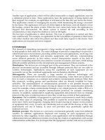
milled for another 24 h and then tape-cast and ‘de-aired’.
The tape-cast BST was punched and stacked to produce
multiple layers. The tapes were then pressed at a pressure
of 35 MPa and a temperature of 70

C for 15 min. A
schematic of this process is shown in Figure 2.4
Ceramic
Powder
Solvent
Deflocculant
Ball-mill
for 24 h
Slurry-1
Plasticizer
Binder
Cyclohexane
Ball-mill for 24 h
Slurry-2
Tape casting
‘De-air’
Tape-cast sheet
Lamination at
0 and 90°
Organic removal
process
Sintering
Multilayed tape-cast BST
⊥

||
Figure 2.4 Flow chart for thick film fabrication using the doctor-blade process.
24 Smart Material Systems and MEMS
2.4.3 Thin films
Thin films of ceramic materials can be fabricated by
using several different approaches. In this section, we
will first describe RF sputtering. Due to its similarity
with the thick film and bulk processing techniques
described above, the sol–gel process for thin films is
also presented here.
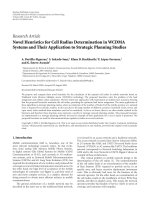
2.4.3.1 Inverted cylindrical magnetron (ICM)
RF sputtering
Figure 2.5 illustrates the ICM sputter gun set-up [26].
This consists of a water-cooled copper cathode, which
houses the hollow cylindrical BST target, surrounded by
a ring magnet concentric with the target. A stainless steel
thermal shield is mounted to shield the magnet from the
thermal radiation coming from the heated table. The
anode is recessed in the hollow-cathode space. The latter
aids in collecting electrons and negative ions, hence
minimizing ‘re-sputtering’ the growing film. Outside
the deposition chamber, a copper ground wire is attached
between the anode and the stainless steel chamber. A DC
bias voltage could be applied to the anode to alter the
plasma characteristics in the cathode/anode space. The
sputter gas enters the cathode region through the space
surrounding the table.
By using the above set-up, Cukauskas et al. [26] were
able to deposit BST films at temperatures ranging from
550 to 800


C. The substrate temperature was maintained
by two quartz lamps, a type-K thermocouple and a
temperature controller. The films were deposited at
135 W to a film thickness of 7000 A

and cooled to
room temperature at 1 atm of oxygen before removing
them from the deposition unit. This was then followed by
annealing the films in 1 atm of flowing oxygen at a
temperature of 780

C for 8 h in a tube furnace.
2.4.3.2 Sol–gel processing technique
The sputtering techniques described above and other
methods, such as laser ablation, MOCVD and hydro-
thermal treatment, require much work, time and high
costs of instrumentations, which lead to a high cost for
the final product. However, large areas of homogenous
films can be obtained by relatively low temperature heat
treatment. The sol–gel method is a technique for produ-
cing inorganic thin films without processing in vacuum,
and offers high purity and ensures homogeneity of the
components at the ‘molecular level’ [29].
In the sol–gel method, the precursor solution of barium
strontium titanates is prepared from barium 2-ethyl hex-
anoate, strontium 2-ethyl hexanoate and titanium tetraiso-
propoxide (TTIP). Methyl alcohol is used as a solvent,
along with acetyl acetonate. A known amount of barium
precursor is dissolved in 30 ml of methyl alcohol and

refluxed at a temperature of about 80

C for 5 h. Strontium
2-ethyl hexanoate is added to this solution and refluxed for
a further 5 h to obtain a yellow-colored solution. Acetyla-
cetonate is added to the solution as a chelating agent, which
prevents any precipitation. This solution is stirred and
refluxed for another 3 h. Separately, a solution of titanium
isopropoxide (TTIP) is prepared in 20 ml of methyl alco-
hol; this solution is added to the barium strontium solution
drop-by-drop and finally refluxed for 4 h at 80

C. Water is
added to the BST solution drop-by-drop in order to initiate
hydrolysis. This solution is refluxed for another 6 h with
vigorous stirring under a nitrogen atmosphere.
For thin-film deposition and characterization, one
could use a substrate such as platinized silicon or a
ceramic. The substrate is immersed in methanol and
dried by nitrogen gas to remove any dust particles. The
precursor solution is coated on the substrate by spin
coating. The latter is carried out by using a spinner
rotated at a rate of 3100 rpm for 30 s. After coating on
the substrate, the films are kept on a hot plate for 15 min
to dry and pyrolyze the organics. This process can be
repeated to produce multilayer films if needed. In such
cases repeated heating after every spin coat is required in
order to successfully ‘burn off’ the organics trapped in
the films. This improves the crystallinity and leads to a
dense sample after multiple coating. To obtain thicker

films, many depositions are required. The films are then
annealed at 700

C for 1 h in air. The annealing tempera-
ture and duration has a significant effect in the film
orientation and properties [30,31].
Figure 2.5 Schematic of the ICM sputter gun set-up [26].
Processing of Smart Materials 25
2.5 SILICON MICROMACHINING
TECHNIQUES
Micromachining is the fundamental technology for the
fabrication of micro electromechanical (MEMS) devices,
in particular, miniaturized sensors and actuators having
dimensions in the sub-millimeter range. Silicon micro-
machining is the most mature of the micromachining
technologies. This process refers to the fashioning of
microscopic mechanical parts out of a silicon substrate
or on a silicon substrate, thus making the structures
three dimensional and hence bringing in new avenues to
designers. By employing materials such as crystalline
silicon, polycrystalline silicon and silicon nitride, a variety of
mechanical microstructures, including beams, diaphragms,
grooves, orifices, springs, gears, suspensions and numerous
other complex mechanical structures, have been fabricated
[32–36].
Silicon micromachining has been a key factor for
the vast progress of MEMS towards the end of the
20th Century. Silicon micromachining comprises two
technologies: bulk micromachining, in which structures
are etched into a silicon substrate, and surface micro-

machining in which the micromechanical layers are formed
from layers and films deposited on the surface. Yet another
but less common method, i.e. LIGA 3D micro-fabrication,
has been used for the fabrication of high-aspect ratio and
three dimensional microstructures for MEMS.
Bulk micromachining, which originated in the 1960s,
has matured as the principal silicon micromachining
technology and has since been used in the successful
fabrication of many microstructures. Presently, bulk
micromachining is employed to fabricate the majority
of commercial devices – pressure sensors, silicon valves
and acceleration sensors. The term ‘bulk micromachin-
ing’ arises from the fact that this type of micromachining
is used to realize micromechanical structures within the
bulk of a single-crystal silicon wafer by selectively
removing the wafer material. The microstructures fabri-
cated by using bulk micromachining may vary in thick-
ness from sub-microns to the full thickness of a wafer
(200 to 500 mm), with the lateral size ranging from microns
to the full diameter of a wafer (usually 75 to 200 mm).
The bulk micromachining technique allows selective
removal of significant amounts of silicon from a substrate
to form membranes on one side of the wafer, a variety
of trenches, holes or other structures. In addition to an
etch process, bulk micromachining often requires wafer
bonding and buried-oxide-layer technologies [37]. How-
ever the use of the latter in bulk micromachining is still
in its infancy. In recent years, a vertical-walled bulk
micromachining techniques, known as single crystal
reactive etching and metallization (SCREAM) which is

a combination of anisotropic and isotropic plasma etching,
hasalsobeenused[36].
Since the beginning of the 1980s, significant interest
has been directed towards micromechanical structures
fabricated by a technique called surface micromachining.
This approach does not shape the bulk silicon, but instead
builds structures on the surface of the silicon by depositing
thin films of ‘sacrificial layers’ and ‘structural layers’ and
by eventually removing the sacrificial layers to release the
mechanical structures. More details on the processing steps
involved in the fabrication of MEMS components using
these techniques will be discussed in Chapter 10. The
dimensions of these surface-micromachined structures
can be several orders of magnitude smaller than bulk-
micromachined structures. The resulting ‘2½-dimensional’
structures are mainly located on the surface of the silicon
wafer and exist as a thin film – hence the ‘half dimension’.
The main advantage of surface-micromachined structures
is their easy integration with IC components, since the
same wafer surface can also be processed for IC elements.
Surface micromachining can therefore be used to build
monolithic MEMS devices.
2.6 POLYMERS AND THEIR SYNTHESIS
Polymers are very large molecules (macromolecules)
made up of a number of small molecules. These small
molecules which connect with each other to build up the
polymer are referred to as monomers and the reaction by
which they connect together is called polymerization.
Recently, a considerable effort is being focused on the
use of polymers in microelectronics and micro electro-

mechanical systems (MEMS). Features that make them
particularly attractive are moldability, conformability,
ease in deposition in the form of thin and thick films,
semiconducting and even metallic behavior in selected
polymers, a choice of widely different molecular struc-
tures and the possibility of piezoelectric and pyroelectric
effects in the polymer side-chain.
For several MEMS devices, the polymers need to have
conductive and possibly piezoelectric or ferroelectric
properties. For these polymers to be used for polymeric
MEMS, they should have the following:
 Strong interfacial adhesion between the various poly-
mer layers.
 Suitable elastic moduli to support the deformation
required in MEMS.
26 Smart Material Systems and MEMS
 Excellent overall dimension stability.
 Long-term environmental stability.
In addition, their processing should help attachment of
nanoceramics and/or conductive phases and formation of
a uniform coating layer. Furthermore, many of these
polymers provide a large strain under an electric field
and thus can be used as actuators for MEMS-based
devices such as micro pumps.
Polymer processing techniques include photopolymer-
ization, electrochemical polymerization and vacuum
polymerization, either stimulated by electron bombard-
ment or initiated by ultraviolet irradiation, or microwave-
assisted polymerization. These methods are also widely
used for processing and curing thin and thick polymer

films on silicon-based electronic components.
Two types of polymers are employed for microma-
chining polymeric MEMS devices: structural polymers
and sacrificial polymers. The structural polymer is
usually a UV-curable polymer with a urethane acrylate,
epoxy acrylate or acryloxysilane as the main ingredient.
Its low viscosity allows easy processing through auto-
matic equipment or by manual methods without the need
to add solvents or heat to reduce the viscosity. It also
complies with all volatile organic compound (VOC)
regulations. It has excellent flexibility and resistance to
fungus, solvents, water and chemicals. The structural
polymer may be used as a backbone structure for build-
ing the multifunctional polymer described below.
It should be pointed out here that the above structural
polymers can also be used to construct sensing and
actuating components for MEMS. Polymer strain gauges
and capacitors can serve as sensing elements for piezo-
resistive and capacitive microsensors [38]. Another impor-
tant point is that as the wafer polymer micro-fabrication
process is being developed for polymer micro devices, the
batch fabrication of polymereric MEMS will not be a
serious concern.
The sacrificial polymer is an acrylic resin containing
50 % silica and is modified by adding crystal violet, as
given in Varadan and Varadan [38]. This composition is
UV-curable and can be dissolved with 2 mol/l of caustic
soda at 80

C. In principle, this process is similar to the

surface micromachining technique used for silicon
devices. However, the process yields 3D structures.
Since only limited sensing and actuation mechanisms
can be obtained using structural polymers by themselves,
a large variety of functional polymers have been used for
MEMS [39]. Some of these functional polymers are listed
in Table 2.4. Such polymers used in smart systems may
contain several functional groups. A ‘Functional group’ is
defined as the atom or group of atoms that defines the
structure of a particular family of organic compounds and,
at the same time, determines their properties. Some
examples of functional groups are the double bond in
alkenes, triple bond in alkynes, the amino (–NH
2
)group,
the carboxyl (–COOH) group, the hydroxyl (–OH) group,
etc. ‘Functionality’ can be defined as the number of such
functional groups per molecule of the compound.
Many polymers used in MEMS are biocompatible and
are thus useful for many medical devices. Applications of
these include implanted medical delivery systems, che-
mical and biological instruments, fluid delivery in
engines, pump coolants and refrigerants for local cooling
of electronic components.
Functional polymer-solid powder composites with
magnetic and magnetostrictive properties have also
been developed for micro devices. For example, the
polymer-bonded Terfenol-D composites showed excel-
lent magnetostrictivity, useful for micro-actuation [41].
The polyimide-based ferrite magnetic composites have

been used as polymer magnets for magnetic micro-
actuators [42].
In addition to being used as sensing and actuating
materials, polymers have also been used for electronics
materials. Polymer transistors have been developed.
Therefore, integrating polymer sensors, actuators and
electronics into polymeric MEMS will be practical for
some special applications.
2.6.1 Classification of polymers
Polymers can be classified, based on their structure (linear,
branched or cross-linked), by the method of synthesis,
physical properties (thermoplastic or thermoset) and by
end-use (plastic, elastomer, fiber or liquid resin).
A linear polymer is made up of identical units
arranged in a linear sequence. This type of polymer has
only two functional groups. Branched polymers are those
Table 2.4 Functional polymers for MEMS.
Polymer Functional Application
property
PVDF Piezoelectricity Sensor/actuator
Polypyrrole Conductivity Sensor/actuator/
electric/connection
Fluorosilicone Electrostrictivity Actuator [40]
Silicone Electrostrictivity Actuator [40]
Polyurethane Electrostrictivity Actuator [40]
Processing of Smart Materials 27
in which there are many side-chains of lined monomers
attached to the main polymer chain at various points.
These side-chains could be either short or long (Figure 2.6).
When polymer molecules are linked with each other

at points, other than their ends, to form a network, the
polymersaresaidtobecross-linked(Figure2.7).Cross-
linked polymers are insoluble in all solvents, even at
elevated temperatures.
Based on their physical properties, polymers may be
classified as either thermoplastic or thermoset. A poly-
mer is said to be a thermoplastic if it softens (flows)
when it is squeezed, or pulled, by a load, usually at a high
temperature, and hardens on cooling. This process of
reshaping and cooling can be repeated several times.
High-density polyethylene (HDPE) or low-density poly-
ethylene (LDPE), poly(vinyl chloride) (PVC) and nylon are
some examples of thermoplastic polymers.
Thermoset polymers, on the other hand, can flow easily
and can be molded when initially produced. Once they are
molded in to their shape, usually by applying heat and
pressure, these materials become very hard. This process
of the polymer becoming an infusible and insoluble mass
is called ‘curing’. Reheating such a thermosetting polymer
just results in the degradation of the polymer and will
distort the object made. Epoxy and phenol formaldehyde
are some examples of thermosetting polymers.
Depending upon their final use, polymers can be
classified as plastic, elastomer, fiber or liquid resin.
When a polymer is formed into hard and tough articles
by the application of heat and pressure, then it is used as
a plastic. When a polymer is vulcanized into rubbery
materials, which show good strength and elongation, it is
used as an elastomer. Fibers are polymers drawn into
long filament-like materials, whose lengths are at least

100 times their diameters. When the polymer is used in
the liquid form, such as in sealants or adhesives, they are
called liquid resins.
2.6.2 Methods of polymerization
There are basically two methods by which polymers can
be synthesized, namely ‘addition’ or ‘chain’ polymeriza-
tion and ‘condensation’ or ‘step-growth’ polymerization.
When molecules just add on to form the polymer, the
process is called ‘addition’ or ‘chain’ polymerization. The
monomer in this case retains its structural identity, even
after it is converted into the polymer, i.e. the chemical
repeat unit in the polymer is the same as the monomer.
When molecules react with each other (with the elimina-
tion of small molecules such as water, methane, etc.),
instead of simply adding together, the process is called
step-growth polymerization. In this case, the chemical
repeat unit is different from the monomer.
2.6.2.1 Addition polymerization
Compounds containing a reactive double bond usually
undergo addition polymerization, also called chain poly-
merization. In this type of polymerization process, a
low-molecular-weight monomer molecule with a double
bond breaks the double bond so that the resulting free
valencies will be able to bond to other similar molecules
to form the polymer. This polymerization takes place in
three steps, namely, initiation, propagation and termina-
tion. This can be induced by a free-radical, ionic or
coordination mechanism. Depending on the mechanism,
there are therefore three types of chain polymerization,
namely, free radical, ionic (cationic and anionic) and

coordination polymerization. The coordination polymer-
ization mechanism is excluded in this present discussion
due to its specialized nature.
2.6.2.2 Free-radical polymerization
There are three steps in polymerization: initiation, pro-
pagation and termination. In this type of polymerization,
the initiation is brought about by the free radicals
produced by the decomposition of initiators, where the
latter break down to form free radicals. Each component
has an unpaired (lone) electron and is called a free
Figure 2.6 The various kinds of branching in polymers:
(a) short; (b) long; (c) star.
Figure 2.7 Illustration of cross-linking in polymers.
28 Smart Material Systems and MEMS
radical. This radical adds to a molecule of the monomer
and in doing so generates another free radical. This
radical adds to another molecule of the monomer to
generate a still larger radical, which in turn adds to yet
another molecule of monomer, and the process continues.
The decomposition of the initiator to form these free
radicals can be induced by heat, light energy or catalysts.
Peroxides, many azo compounds, hydroperoxides and
peracids are the most commonly used initiators. The
latter can also be decomposed by UV light. The rate of
decomposition in this case depends mainly on the inten-
sity and wavelength of radiation and not so much on the
temperature. A polymerization reaction initiated by UV
light falls under the category of photoinitiated polymer-
ization. The reaction in such a case may be expressed as
follows

PI þ hn ÀÀÀ! R

0
ð2:6Þ
where PI represents the photoinitiator, and R

0
is the
reactive intermediate from the UV cleavage of PI.
UV curing is therefore based on photoinitiated
polymerization which is mediated by photoinitiators.
These photoinitiators are required to absorb light in the
UV–visible spectral range, generally 250–550 nm, and
convert this light energy into chemical energy in the
form of reactive intermediates, such as free radicals
and reactive cations, which subsequently initiates the
polymerization.
During the propagation step, the radical site on the
first monomer unit reacts with the double bond of a
‘fresh’ monomer molecule, which results in the linking
up of the second monomer unit to the first and the
transfer of the free radical onto the second monomer
molecule. This process, involving the attack on a fresh
monomer molecule, which in turn keeps adding to the
growing chain, is called propagation. The chain keeps
propagating as far as the monomer is available. This step
can also end when the free-radical site is ‘killed’ by some
impurities or by the termination process.
The propagation step can be represented as follows:
M


1
þ M ÀÀÀ! M

2
ð2:7Þ
where M represents the monomer molecule, and
M

1
M

n
represent reactive molecules.
The last step in the polymerization reaction is called
termination. In this step, any further addition of the mono-
mer units to the growing chain is stopped and the growth
of the polymer chain is inhibited. The decomposition of
the initiator results in the formation of a large number of
free radicals. Depending on factors such as temperature,
time and monomer and initiator concentrations, there exists
a chance when the growing chains collide against each
other. This can occur in two ways:
 Termination by combination – the chain terminates by
the simple formation of a bond between two radicals.
 Termination by disproportionation – a proton is trans-
ferred and a double bond is formed.
These reactions can be represented as follows:
M


x
þ M

y
ÀÀÀ! M
xþy
ðcombinationÞð2:8Þ
M

x
þ M

y
ÀÀÀ! M
x
þ M
y
ðdisproportionationÞð2:9Þ
where M
xþy
is the stable polymer molecule containing x þ y
monomer units, while M
x
and M
y
arealsostablepolymer
molecules with x and y monomer units, respectively.
Some common monomers that can be polymerized by
using free-radical polymerization are listed in Table 2.5.
2.6.2.3 Cationic polymerization

Ionic polymerization involves the breaking down of the
p-electron pair of the monomer. This is not done by free
radicals but by either a positive or negative ion. If the
active site has a positive charge (i.e. a carbonium ion),
then it is called cationic polymerization. Monomers
which have an electron-donating group are the most
suitable for cationic polymerization, for example, alkyl
vinyl ethers, vinyl acetals, isobutylene, etc.
Initiation in this case can be achieved by using proto-
nic acids and Lewis acids. The latter usually require a
‘co-catalyst’ such as water or methyl alcohol. Here, a
proton is introduced into the monomer. This proton pulls
the p-electron pair towards it and this is how the positive
Table 2.5 Examples of monomers polymerized
by using free-radical polymerization.
Monomer Structure
Ethylene CH
2
=CH
2
Butadiene CH
2
=CH–CH=CH
2
Styrene CH
2
=CH–C
6
H
5

Vinyl chloride CH
2
=CH–Cl
Vinylidene chloride CH
2
–CCl
2
Acrylic acid CH
2
=CH–COOH
Methyl methacrylate CH
2
–C(CH
3
)COOCH
3
Processing of Smart Materials 29
charge moves to the other end of the monomer, hence
resulting in the formation of a carbonium ion:
C þXH
ÀÀÀ*
)ÀÀÀÀ
H
È
X
Â
C ðion-pair formationÞð2:10Þ
H
È
X

Â
C þ M ÀÀÀ! HM
Â
X
È
C ðinitiationÞð2:11Þ
where C is the catalyst, XC the co-catalyst and M the
monomer.
Propagation of the cationic polymerization reaction
occurs as the carbonium ion attacks the p-electron pair of
the second monomer molecule. The positive charge is
then transferred to the farther end of the second mono-
mer, and thus a chain reaction is started:
HM
È
X
Â
C þMÀÀ À! HMM
È
X
Â
C ðpropagationÞð2:12Þ
Termination can occur by anion–cation recombination,
resulting in an ester group. Termination can also occur by
splitting of the anion. This occurs by reaction with trace
amounts of water:
HM
n
M
È

X
Â
C þM ÀÀÀ! HM
n
M þ H
È
X
Â
C ðterminationÞ
ð2:13Þ
HM
n
M
È
X
Â
C ÀÀÀ! HM
n
M þ H
È
X
Â
C
ðchain transfer to monomerÞð2:14Þ
2.6.2.4 Anionic polymerization
If the active site has a negative charge (i.e. a carbanion),
then the process is called anionic polymerization. Mono-
mers capable of undergoing anionic polymerization are
isoprene, styrene and butadiene.
Initiation takes place in the same way as in cationic

polymerization, except that here a carbanion is formed.
The general initiators used in this case are the alkyl
and aryl derivatives of alkali metals such as triphenyl
methyl potassium and ethyl sodium. Propagation then
proceeds with the transfer of the negative charge to
the end of the monomer molecule. Termination is not
always a spontaneous process, and unless some impu-
rities are present or some strongly ionic substances
are added, termination does not occur. So, if an inert
solvent is used and if impurities are avoided, the reac-
tion proceeds up until all of the monomer is consumed.
Once this is achieved, the carbanions at the end of the
chain still remain active and are considered as ‘living’;
polymers synthesized by using this method are known
as ‘living polymers’. This technique is useful for pro-
ducing block copolymers.
IA ÀÀÀ! I
È
A
Â
ðion- pair formationÞð2:15Þ
A
Â
I
È
þM ÀÀÀ! AM
Â
I
È
ðinitiationÞð2:16Þ

AM
Â
I
È
þM ÀÀÀ! AM M
Â
I
È
ðpropagationÞð2:17Þ
AM
n
M
Â
I
È
þHA ÀÀÀ! AM
n
MH þA
Â
I
È
ðterminationÞ
ð2:18Þ
where IA is the initiator and HA is a protonating agent,
2.6.2.5 Step-growth polymerization
Step polymerizations are carried out by the stepwise
reaction between the functional groups of the monomers.
In such polymerizations, the size of the polymer chains
increases at a relatively slow rate from monomer to
dimer, trimer, tetramer, pentamer and so on:

Monomer þMonomer (Dimer)
Dimer þMonomer (Trimer)
Dimer þDimer (Tetramer)
Trimer þDimer (Pentamer)
Trimer þTrimer (Hexamer)
Any two molecular species can react with each other
throughout the course of the polymerization until, even-
tually, large polymer molecules consisting of large num-
bers of monomer molecules have been formed. These
reactions take place when monomers containing more than
two reactive functional groups react. Typical condensation
polymers include polyamides, polyesters, polyurethanes,
polycarbonates, polysulfides, phenol formaldehyde, urea
formaldehyde and melamine formaldehyde.
When a pair of bifunctional monomers (dicarboxylic
acid/diamine or dialcohol/dihalide) undergoes polycon-
densation, it is called an AA–BB-type polycondensation:
nAÀA þ nBÀB ÀÀÀ! AÀÀ½ ABÀÀ
2nÀ1
B þbyproduct
ð2:19Þ
When a single bifunctional monomer undergoes
self-condensation, it is known as an A-B type polycon-
densation.
nAÀB ÀÀÀ! BÀÀ½ ABÀÀ
nÀ1
A þbyproduct ð2:20Þ
30 Smart Material Systems and MEMS
If in the AA–BB type of polycondensation, one of the
monomers has a functionality of three or more, it forms a

3D network. Figure 2.8 illustrates the formation of net-
works in polymers with a functionality of three or higher,
while Table 2.6 shows some examples of functionality in
monomer compounds.
Some of the common monomers that can be polymer-
ized by using step-growth polymerization are listed in
Table 2.7.
2.7 UV RADIATION CURING
OF POLYMERS
Radiation curing refers to radiation as an energy source
to induce the rapid conversion of specially formulated
100 % reactive liquids into solids by polymerizing and
cross-linking functional monomers and oligomers (usually
liquid) into a cross-linked polymer network (usually
solid) [43].
The radiation energy could be from electron beams,
X-rays, g-rays, plasmas, microwaves and, more commonly,
ultraviolet (UV) light. UV radiation curing has also been
extensively used in MEMS, photoresist patterning and
building flexible polymer structures (both planar and
three-dimensional) (UV-LIGA, microstereolithography,
etc.). Advantages of using radiation curing include the
following:
. It has a high processing speed and hence a high
productivity.
. The processes are very convenient and economical,
plus since most comprise ‘one pack compositions’,
they can be dispensed automatically.
. There is very low heat generation and so heat-sensitive
substrates can be used.

. Lower energy and space requirements than conven-
tional curing systems.
. Since the organic emission levels are very low, this
treatment is ‘eco-friendly’.
. Low capital costs, especially if UV is used as the
curing ‘stimulant’.
2.7.1 Relationship between wavelength
and radiation energy
Typical average energies from the homolytic cleavage of
selected chemical bonds in organic molecules are shown
in Table 2.8 [44]. The radiation wavelengths that can
potentially break these bonds are given by Planck’stheory.
(a)
(b)
(c)
(d)
Figure 2.8 Illustration of the formation of networks in polymers with a functionality greater than two: (a,b) functional groups are at
the ends of the line segments; (c) a chain of a trifunctional polymer; (d) a network of a tetrafunctional polymer.
Table 2.6 Functionality of some monomer compounds.
Compound Chemical formula Functional Number of Functionality
group functional groups
Ethyl alcohol CH
3
CH
2
OH –OH 1 Monofunctional
Hexamethylene H
2
NCH
2

(CH
2
)
4
CH
2
NH
2
–NH
2
2 Bifunctional
diamine
Maleic acid HOOCCH
2
CH(OH)COOH –COOH, –OH 3 Trifunctional
Gallic acid HOOCC
6
H
2
(OH)
3
–COOH, –OH 4 Tetrafunctional
Processing of Smart Materials 31
Planck developed his theory of ‘black-body radiation’
on the basis of a postulate that radiation possessed
particulate properties and that the particles, or photons,
of radiation of a specific frequency, n, had associated
with them a fixed energy, e, given by the relationship
e ¼hn, where h is known as the Planck constant
(6:626 076 Â10

À34
J s) and n ¼ c=l, in which c is the
speed of light (3 Â 10
8
m/s) and l is the wavelength.
Figure 2.9 illustrates the relevant ranges in the electro-
magnetic spectrum. This shows that photons at wave-
lengths within the UV range possess enough energy to
break the bonds listed in the table and these undergo
rearrangements to form polymer networks [45].
2.7.2 Mechanisms of UV curing
UV curing is based on photoinitiated polymerization,
which is mediated by photoinitiators. These absorb
UV light and convert the (light) energy into chemical
energy in the form of reactive intermediates, such as
free radicals and reactive cations, which subsequently
initiate the polymerization. Typical photopolymer for-
mulations contain a photoinitiator system, monomers
and oligomers (or a polymer or polymers) to provide
specific physical and/or processing properties. They
mayalsocontainavarietyofadditivestomodifythe
physical properties of the light-sensitive compositions
or the final properties of the cured photopolymers.
The photopolymerization reactions fall into two cate-
gories, i.e. radical photopolymerization and cationic
Table 2.7 Some of the polymers that can be
prepared by using step-growth polymerization.
Polymer Chemical formula
Nylon 6
NH C

O
(CH
2
)
5
n
Polycarbonate
OC
CH
3
CH
3
C
O
n
Poly(butylene
(CH
2
)
4
OC
O
C
O
n
terephthalate)
Table 2.8 Energies and corresponding wavelengths
for the homolytic fission of typical chemical bonds [44].
Bond Energy kcal/mol l (nm)
C=C 160 179

C–C 85 336
C–H95–100 286–301
C–O80–100 286–357
C–Cl 60–86 332–477
C–Br 45–70 408–636
O–O 35 817
O–H85–115 249–336
200 300 400 500 600 700 800 900
10
–6
10
–4
10
–2
10 10
2
10
4
10
6
10
8
10
10
10
12
Cosmic
rays
Gamma
rays

X-rays
Infrared
rays
‘Hertzian’
waves
Radio
waves
Vacuum UV Far UV Near UV
Ran
g
e for UV curin
g

Visible
Near IR
Figure 2.9 The electromagnetic spectrum (wavelengths in nanometers) [11].
32 Smart Material Systems and MEMS
photopolymerization. Generally, acrylates are associated
with free-radical polymerization while epoxies are typi-
cal of cationic curing. The most commonly used reactive
monomeric materials are low-molecular-weight unsatu-
rated acrylate or methacrylate monomers that can be
made to cross-link with the use of a radical-generating
photoinitiator. The practical applications of cationic-
initiated cross-linking of monomeric materials with
epoxy and/or vinyl ether functionalities have signifi-
cantly increased with the development of new UV-
sensitive, high-efficiency photoinitiators which generate
cationic species (e.g. strong acids). Table 2.9 gives a
comparison of the characteristics of cationic and free-

radical curing, showing their relative merits and demer-
its. In this table, moisture inhibition refers to the ability
of a formulation to cure in the presence of atmospheric
moisture, while post-irradiance cure refers to curing
taking place after the light source has been removed.
For free-radical curing in air, surface curing lags behind
bulk curing, which is known as ‘oxygen inhibition’. This
lag results from competition at the surface between
oxygen molecules and free radicals for the monomer
sites. A through cure of cationic systems is recommended
since free radicals have a limited lifetime.
Once the photoinitiator (PI) absorbs light, it is raised to
an electronically excited state, PI
*
. The lifetimes of the
PI* states are short, generally less than 10
À6
s. During
this time, the PI
*
state may be affected by the one of the
following possibilities: (i) it may decay back to the PI
state with the emission of light and/or heat; (ii) it may
attain a (further) excited state following quenching by
oxygen, monomer or other quenching agents; (iii) it
may disintegrate by a chemical reaction, yielding the
initiator species, R
0
[46].
The rate of initiation (R

i
) is expressed as the rate of
formation of PI
*
, which corresponds to the number of
photons absorbed by the PI per unit time:
R
i
¼ I
abs
Ff ð2:21Þ
where the term I
abs
corresponds to the intensity of light
absorbed by the PI, F is the fraction of PI
*
that yields
initiator species, and f is the fraction of initiator which
initiates polymerization. I
abs
is related to the incident
light intensity (I
0
), the number of photons incident to the
system per unit time and area and the absorbance (A)of
the PI, according to the Beer-Lambert law:
I
abs
¼ I
0

ð1 À 10
ÀA
Þ
where A ¼ e dc ð2:22Þ
where d is the pathlength of light (or film thickness), e is the
molar absorptivity of the PI and c is the PI concentration.
It is desirable that the rate of initiation, R
i
, be uniform
throughout the system and to be high enough for efficient
utilization of the light energy. For example, internal
stresses arising from non-uniform cross-linking adversely
affect adhesion to the substrate and mechanical properties,
such as tensile strength. From Equation (2.22), one can
also see that the non-uniformity of the absorption increases
with the absorbance A. Therefore, the appropriate PI
concentration, molar absorptivity of PI and the value of
absorbance of the system are very important in order to
optimize a monomer system for UV curing [46].
2.7.3 Basic kinetics of photopolymerization
Since the rate of polymerization is an important parameter
in characterizing polymer curing, the curing profile can be
predicted from this. The kinetics of photopolymerization
presented below should prove helpful in understanding
how to calculate the rate of polymerization.
2.7.3.1 Radical photopolymerization
Radical photopolymerization is a chain reaction which
proceeds according to the following steps:
PI þ hn ÀÀÀ! R


ð2:23Þ
R

þ M ÀÀÀ!
k
i
RM

1
Photoinitiation ð2:24Þ
RM

1
þ M ÀÀÀ!
k
p
RM

2
; etc: Propagation ð2:25Þ
RM

nÀ1
þ M ÀÀÀ!
k
p
RM

n
Propagation ð2:26Þ

RM

n
þ RM

m
ÀÀÀ!
k
t
RM
mþn
Termination ð2:27Þ
Table 2.9 Comparison of free-radical curing versus
cationic curing [45].
Property Free-radical Cationic
curing curing
Cure speed Faster Slower
Oxygen inhibition Yes No
Adhesion ‘Problems’ Excellent
Toxicity Skin irritation Acceptable
Moisture inhibition No Yes
Post-irradiation cure No Yes
Formulation latitude Good Limited
Through cure Fair Good
Viscosity Higher Lower
Cost Moderate Higher
Processing of Smart Materials 33
where PI represents the photoinitiator, RM
mþn
is the

stable polymer molecule and k
i
, k
p
and k
t
are the rate
constants for initiation, propagation and termination,
respectively.
The rate of photochemical initiation is expressed as
follows:
R
i
¼ 2FI
abs
ð2:28Þ
where I
abs
is the intensity of absorbed light in moles of
light quanta per liter and second and F, referred to as the
quantum yield for initiation, is the number of propagating
chains initiated per light photon absorbed. The factor of
‘2’ indicates that two radicals are produced per molecule
undergoing photolysis. The maximum value of F is 1 for
all photoinitiated polymerizations.
Monomers are consumed by the initiation reaction, as
well as by propagation reactions. The rate of change in
monomer concentration by polymerization is expressed
as follows:
À

d½M
dt
¼ R
i
þ R
p
ð2:29Þ
where R
i
and R
p
are the rates of initiation and propaga-
tion, respectively. For a process producing high-molecular-
weight polymers, the number of monomers reacting in the
initiation step is far less than that in the propagation step.
Thus, Equation (2.29) can be simplified as follows:
À
d½M
dt
¼ R
p
ð2:30Þ
Assume that the rate constants for all of the propaga-
tion steps are the same, the polymerization rate can be
expressed by the following:
R
p
¼ k
p
½M½M


ð2:31Þ
where [M] is the monomers concentration and [M

] is the
total concentration of all chain radicals.
The polymerization rate cannot be directly obtained
from Equation (2.31) since it is difficult to measure the
radical concentrations quantitatively, which are very low
($ 10
À8
M). In order to eliminate [M

] from Equation
(2.31), we use a steady-state assumption that the con-
centration of radicals increases initially but then reaches
a constant steady-state value within a very short time.
This means that the rates of initiation, R
i
, and termina-
tion, R
t
, of the radicals are equal, or:
R
i
¼ R
t
¼ 2k
t
½M



2
ð2:32Þ
where the factor of ‘2’ in the above equation represents
the fact that the radicals are ‘destroyed’ in pairs. By
rearranging Equation (2.32), the concentration of the
radicals is given by:
½M

¼
R
i
2k
t

1=2
ð2:33Þ
and then by substituting Equation (2.33) into Equation
(2.31), we obtains:
R
p
¼ k
p
½M
R
i
2k
t


1=2
ð2:34Þ
A combination of Equations (2.28) and (2.34) then
yields:
R
p
¼ k
p
½M
FI
abs
k
t

1=2
ð2:35Þ
and by using Equation (2.22), the expression for R
p
becomes:
R
p
¼ k
p
½M
FI
0
ð1 À 10
Àedc
Þ
k

t
!
1=2
ð2:36Þ
2.7.3.2 Cationic photopolymerization
The process of cationic photopolymerization can be
generalized as follows:
PI þhn ÀÀÀ! H
þ
X
À
ð2:37Þ
H
þ
X
À
þM ÀÀÀ!
k
i
HM
þ
1
X
À
Photoinitiation ð2:38Þ
HM
þ
1
X
À

þM ÀÀÀ!
k
p
HM
þ
2
X
À
;etc: Propagation ð2:39Þ
HM
þ
nÀ1
X
À
þM ÀÀÀ!
k
p
HM
þ
n
X
À
Propagation ð2:40Þ
HM
þ
n
X
À
ÀÀÀ!
k

t
HM
n
X Termination ð 2:41Þ
The reaction rates for initiation, propagation and termi-
nation are expressed as follows:
R
i
¼ FI
abs
ð2:42Þ
R
p
¼ k
p
½HM
þ
X
À
½Mð2:43Þ
R
t
¼ k
t
½HM
þ
X
À
ð2:44Þ
where [HM

þ
X
À
] is the total concentration of the reactive
centers. Supposing that the steady-state assumption is
34 Smart Material Systems and MEMS
also valid for cationic photopolymerization, one can get
the following:
½HM
þ
X
À
¼
FI
abs
k
t
ð2:45Þ
A combination of Equations (2.43) and (2.45) yields:
R
p
¼
k
p
FI
abs
½M
k
t
ð2:46Þ

This is the rate of polymerization for cationic photo-
polymerization. R
p
can also be expressed in terms of I
0
,
which is as follows:
R
p
¼ k
p
½M
FI
0
ð1 À 10
Àedc
Þ
k
t
ð2:47Þ
2.8 DEPOSITION TECHNIQUES FOR
POLYMER THIN FILMS
A brief list of the polymeric materials commonly used
in the context of various microsystems is presented in
Table 2.10. Polypyrrole is one candidate for a sorbent
thin-film material. Chemical oxidation as a means of
depositing these conducting polymers onto host mem-
branes has been shown to be useful [47]. In this method,
the host PVDF film is ‘pre-wet’ in a 50 % ethanol solution
and then dipped into the monomer (pyrrole) solution. The

‘superficial’ solution is ‘blot dried’ with filter paper. This
coated material is then dipped in an oxidant solution (e.g.
ferric chloride hexahydrate) for chemical polymerization.
A similar approach has been reported by de Lacy Costello
et al. [48], where ferric nitrate solution was used for
polymerization.
To deposit polymer thin films without affecting their
chemical integrity and physico-chemical properties, the
pulsed laser deposition technique has been recently used
[49]. A patterned deposition is possible by incorporating
an x–y positioning stage in this approach. These authors
[49] have deposited a fluoroalcoholpolysiloxane (SXFA)
polymer under vacuum onto piezoelectric substrates in
this way. In yet another instance, UV-induced graft
copolymerization with 4-vinylpyridine has been used
for surface modification of PVDF for the electroless
deposition of nickel [50]. This method enhanced the
adhesion of nickel to the PVDF by interfacial charge-
transfer interactions between the grafted polymer chains
and the deposited metals, the spatial distribution of the
grafted chains into the metal matrix and the covalent
‘tethering’ of the grafted chains on the PVDF surface.
Processing techniques involved in the fabrication of
polymer MEMS are described in Chapter 11.
2.9 PROPERTIES AND SYNTHESIS
OF CARBON NANOTUBES
Over the last few years there has been an increasing trend
to further miniaturize the sensors/actuators from the
micro to the nano scale. This is due to some outstanding
properties that these nano-scale materials can offer over

conventional bulk materials. One such nano-scale mate-
rial is the carbon nanotube (CNT). From their unique
electronic properties and thermal conductivities higher
than diamond to mechanical properties where the stiff-
ness, strength and resilience exceed any current material,
carbon nanotubes offer tremendous opportunities for the
development of fundamentally new material systems. In
particular, the exceptional mechanical properties of car-
bon nanotubes, combined with their low density, offer
much scope for the development of nanotube-reinforced
composite materials. The potential for nanocomposites,
reinforced with carbon nanotubes, having extraordinary
specific stiffness and strength properties, represent tremen-
dous opportunities for applications in the 21st Century.
The research towards exploring the various special
properties of carbon began in the mid-1980s, when
Smalley and coworkers discovered the fullerenes [51],
which are cage-like structures of carbon atoms having
hexagonal and pentagonal faces. The first closed convex
structure formed is the C
60
‘buckyball’ structure. The
other forms of carbon-based materials that can exist in
different forms are ‘Diamond’ and the ‘graphite’ sheets.
In 1991, Iijima [52] discovered yet another form of
carbon-based material, which he named as ‘carbon nano-
tubes’. All of these forms are shown in Figure 2.10.
CNTs, due to their superior properties, have immense
potential for use in many structural applications. A single
layer of CNTs can achieve 50 times the tensile strength

of conventional steel [53], while the mass density of
CNTs is only 1/6 that of steel. These properties highlight
the promising role of CNTs in applications involving
nanomaterials and nanodevices. Theoretically, the tensile
modulus and strength of a graphene layer can reach up to
1 TPa and 200 GPa, respectively.
In addition to the exceptional mechanical properties
associated with carbon nanotubes, they also possess
superior thermal and electric properties. They are ther-
mally stable up to 2800

C in vacuum, have a thermal
Processing of Smart Materials 35
Table 2.10 Polymeric materials commonly used in various microsystems.
Polymer Acronym Chemical formula
General properties
Polyethylene PE
CH
2
CH
2
n
Excellent chemical resistance, low cost, good electrical insulation
properties, clarity of thin films, easy processability
Poly(vinyl chloride) PVC
CH
CH
2
n
Cl

Excellent electrical insulation over a range of frequencies,
good fire-retardant properties, resistance to weathering
Poly(vinylidene fluoride) PVDF
C
CH
2
n
F
F
Piezoelectric and pyroelectric properties,
excellent resistance to ‘harsh’ environments
Polytetrafluoroethylene PTFE
C
C
n
F
F
F
F
High heat resistance, high resistance to chemical agents and
solvents, high ‘anti-adhesiveness’, high dielectric properties,
low friction coefficient non-toxic.
Poly(vinyl acetate) PVAC
CH
O
CH
2
C
O
CH

3
n
Good adhesive properties.
Poly(vinyl alcohol) PVAL
CH
OH
CH
2
n
Good adhesive properties, water absorption, heat resistance,
electrical insulation
Polyamide Nylon 6
NH C
O
(CH
2
)
5
n
Very good abrasion resistance, excellent resistance
to hydrocarbons
Polystyrene PS
CH CH
2
n
Optical properties (transparency),
ease of coloring and processing
Polybutyleneterephthalate PBT
(CH
2

)
4
OC
O
C
O
n
Good dimensional stability in water, high mechanical strength,
low water absorption
Poly(ether ether ketone) PEEK
OC
O
n
Hydrolysis resistance, good resistance to acids
Polycarbonate PC
OC
CH
3
CH
3
C
O
n
High impact strength, low moisture absorption, good heat resistance,
good rigidity and electrical properties, high light transmission,
high creep resistance
Poly(methyl methacrylate) PMMA
C
C
CH

3
CH
2
O
OCH
3
n
Excellent weatherability, combination of stiffness, density and
moderate toughness, elasticity, optical properties
Polyimide PI
C
N
CC
N
C
O
O
O
O
n
Elasticity
Silicone rubber
Si
CH
3
CH
3
O
n
Elasticity

Polysulfone PSU
SO
2
n
Good for molding
Polypyrrole PPy
N
n
Electroactive, conducting
Polydimethylsiloxane PDMS
Si
CH
3
CH
3
O
n
Elasticity and biomedical compatibility
Polyaniline PANI
NH
n
Electroactive, conducting
conductivity about twice as high as diamond and an
electric-current-carrying capacity 1000 times higher than
copper wire. These exceptional properties have been inves-
tigated for devices such as field-emission displays, scan-
ning probe microscopy tips and microelectronic devices.
The size, mechanical strength and electrical properties
of nanotubes are highly dependent on the atomic archi-
tecture. It has been reported that armchair nanotubes

exhibit better ductility and electrical conductivity than
zigzag nanotubes. Schematics of these two forms are
CNTs shown in Figure 2.11 exist in two different forms.
A single-walled carbon nanotube (SWCNT) has a hol-
low structure formed by covalently bonded carbon atoms
and can be imagined as a rectangular graphene sheet
rolled from one side of its longest edge to form a
cylindrical tube. Hemispherical caps seal both ends of
the tube as shown in Figure 2.10. For multi-walled
carbon nanotubes (MWCNTs), a number of graphene
layers are co-axially rolled together to form a cylindrical
tube (Figure 2.11). The spacing between the graphene
layers is about 0.34 nm. In other words, an MWCNT is
thought to be made up of nested shells of cylinders with
weak interlayer interactions. These values have been
widely used to interpret the mechanical properties of
single-walled and multi-walled nanotubes. The typical
dimensions of SWCNTs are shown in Table 2.11.
It has also been observed that the majority of carbon
nanotubes exhibit chirality [54] (Figure 2.12). In other
words, the been hexagonal carbon orientation with
respect to the tubular axis could be different for different
carbon nanotubes. The properties of CNTs depend lar-
gely on their diameters and chirality. Carbon nanotubes
have extraordinary mechanical, thermal and electrical
properties due to their unique carbon structure, as well
as their nano-size scale [55]. Wong et al. [56] reported
the average Young’s modulus value of MWCNTs, deter-
mined by atomic force microscopy (AFM) measure-
ments, to be 1.28 Æ 0.59 TPa, which is the largest of

any known material. Wildo
¨
er et al. used scanning tunnel-
ing microscopy (STM) to measure the conductivities of
individual carbon nanotubes and found that these depend
on the chiral angle and diameter [55].
Figure 2.10 Different forms of carbon-based materials. Reprinted from Composites Part B Engineering, vol 35 (2), pp. 95–101,
Copyright 2004, with permission from Elsevier
Figure 2.11 Different forms of carbon nanotubes: (a) arm-
chair; (b) zig-zag. Reprinted from Composite Science &
Technology, 61, 1899–1912, Copyright 2001, with permission
from Elsevier
Table 2.11 Key geometric parameters of
single-walled carbon nanotubes.
Parameter Range of values
Thickness 0.0066–0.34 nm
Diameter 0.40–100 nm
Length 1 nm–1 mm
38 Smart Material Systems and MEMS
The features (size, single- or multi-walled, helicity,
etc.) of carbon nanotubes are also determined by the
method of preparation. There are several methods for the
synthesis of carbon nanotubes. Arc discharge and laser
vaporization of a graphite electrode in the presence of
metal catalysts were the earliest methods used to synthe-
size CNTs [57]. However, both of these methods require
reaction temperatures higher than 3000

C, which is
incompatible with modern IC fabrication. Another lim-

itation is the high production cost due to the complex
equipment required and the low deposition rate [58]. In
recent years, pyrolysis of hydrocarbon (e.g. acetylene,
methane, etc.) vapors over transition metals incorporated
on a catalyst support has attracted much research interest
because of the simplicity of the equipment and reprodu-
cibility of the product in comparison with other methods.
Another method to produce high-quality carbon nano-
tubes is the use of microwave CVD. Compared with the
conventional thermal filament CVD method, microwave
CVD has much faster heating and cooling times and
higher yields of nanotubes. By optimization, this approach
is expected to result in up to 90 % yields and a large-scale
production capability [59]. Techniques for the purification
and functionalization of nanotubes for nanocomposites
and MEMS have also been developed [59].
Carbon nanotubes are regarded as promising filler
materials for a new generation of high-performance
nanocomposites because of their exceptionally high
Young’s modulus [60], bending strength and low density.
The use of physical bonding and chemical bonding
represent two approaches for preparing composites of
nanotubes. In the former method, the CNTs are added to
a solvent, e.g. chloroform, toluene, ethanol, etc. and a
high-power ultrasonic probe is used to disperse the
system. Then, the dispersed nanotubes are blended with
the host material. Composite films can be deposited by
drop- and spin-coating on various substrates. In this
method, the carbon nanotubes are only physically bonded
to the host material. Because of the pure carbon compo-

sition and their stable structures, carbon nanotubes are
insoluble in all organic solvents. This makes it extremely
difficult to explore their properties and applications.
Furthermore, because the high surface energies make
carbon nanotubes easy to agglomerate (due to their nano-
size dimensions, composite processing is still limited to
bench-top levels and has been hampered by the high
viscosities of available matrix materials, lack of good
dispersion techniques and excessive porosity [61].
To overcome this problem, chemical modification by
functionalization of the carbon nanotube surface has
been pursued [62]. It has been reported that functiona-
lized nanotubes can form stable and uniform colloidal
dispersions with some solvents. This can be explained by
the electrostatic repulsion resulting from the functional
groups attached to the surfaces of the nanotubes. Thus,
well-dispersed colloidal systems are required for in situ
polymerization. The functional groups attached to the
surfaces of the nanotubes are able to react with functional
monomers to form a chemically bonded UV-curable
polymer. The ‘functionalization yield’ can be enhanced
by using a phase-transfer catalyst at room temperature
[63]. A UV-curable polymer with chemically bonded
nanotubes can be synthesized by a three-step in situ
polymerization. Since UV curing is one of the preferred
methods of MEMS fabrication, especially by microster-
olithography, those materials are likely to have many
Armchair
Zig-Zag
ma

2
na
1
Chiral vector
a
1
a
2
Figure 2.12 Schematic showing the formation of a carbon nanotube from a rolled graphite sheet. Reprinted from Composite
Science & Technology, 61, 1899–1912, Copyright 2001 with permission from Elsevier
Processing of Smart Materials 39
potential applications. Design modeling and fabrication
of CNT based microsystems will be presented in later
chapters.
REFERENCES
1. G.T.A. Kovacs, N.I. Maluf and K.E. Petersen, ‘Bulk micro-
machining of silicon’ Proceedings of the IEEE, 86, 1536–
1551 (1998).
2. J.M. Bustillo, R.T. Howe and R.S. Muller, ‘Surface micro-
machining for microelectromechanical systems’, Proceed-
ings of the IEEE, 86, 1552–1574 (1998).
3. H. Guckel, ‘High-aspect-ratio micromachining via deep X-ray
lithography’, Proceedings of the IEEE, 86,1586–1593 (1998).
4. Y. Xia and G.M. Whitesides, ‘Soft lithography’, Angewandte
Chemie, International Edition, 37, 550–575 (1998).
5. V.K.Varadan and V.V. Varadan, ‘Three dimensional poly-
meric and ceramic MEMS and their applications’, Proceed-
ings of SPIE, 2722, 156–164 (1996).
6. K. Ikuta and K. Hirowatari, ‘Real three dimensional micro-
fabrication using stereo lithography and metal molding’,in

Proceedings of the IEEE: MEMS’93, IEEE, Piscataway, NJ,
USA, pp. 42–47, (1993).
7. T. Katagi and N. Nakajima, ‘Photoforming applied to fine
machining’,inProceedings of the IEEE: MEMS’93, IEEE,
Piscataway, NJ, USA, 173–178, (1993).
8. C.S. Taylor, P. Cherkas, H. Hampton, J.J. Frantzen, B.O.
Shah, W.B. Tiffany, L. Nanis, P. Booker, A. Salahieh and R.
Hansen, ‘A spatial forming – a three dimensional printing
process’,inProceedings of the IEEE: MEMS’94, IEEE,
Piscataway, NJ, USA, pp. 203–208 (1994).
9. G. Thornell and S. Johansson, ‘Microprocessing at the
fingertips’, Journal of Micromechanical and Microengineer-
ing, 8, 251–262 (1998).
10. J.W. Gardner, V.K. Varadan and O.O. Awadelkarim, Micro-
sensors MEMS and Smart Devices, John Wiley & Sons, Ltd,
London, UK (2002).
11. V.K. Varadan, X. Jiang and V.V. Varadan, Microstereolitho-
graphy and other Fabrication Techniques for 3D MEMS,
John Wiley & Sons, Ltd, London, UK (2001).
12. L.E. Larson, ‘Microwave MEMS technology for next-gen-
eration wireless communications’, IEEE MTT-S Interna-
tional Symposium Digest, 3, 1073–1076 (1999).
13. L.T. Romankiw, ‘A path: from electroplating through litho-
graphic masks in electronics to LIGA in MEMS’, Electro-
chimica Acta, 42, 2985–3005 (1997).
14. C.H. Ahn and M.G. Allen, ‘Micromachined planar inductors
on silicon wafers for MEMS applications’, IEEE Transac-
tions on Industrial Electronics, 45, 866–876 (1998).
15. H.O. Pierson, Handbook of Chemical Vapor Deposition
(CVD): Principles, Technology and Applications, 2nd Edn,

Noyles Publications, New York, NY, USA (1999).
16. A. Ohta, S. Bhansali, I. Kishimoto and A. Umeda, ‘Devel-
opment of TiNi shape memory alloy film deposited by
sputtering from separate Ti and Ni targets’, Proceedings of
SPIE, 3512, 138–145 (1998).
17. T. Honda, K.I. Arai and M. Yamaguchi, ‘Basic properties of
magnetostrictive actuators using Tb–Fe and Sm–Fe thin
films’, IEICE Transactions on Electronics, E80-C, 232–238
(1997).
18. L.C. Chin, V.V. Varadan and V.K. Varadan, ‘Hybrid finite
element formulation for periodic piezoelectric arrays sub-
jected to fluid loading’, International Journal of Numerical
Methods in Engineering, 37, 2987–3003 (1994).
19. V.K. Varadan, K.J. Vinoy and K.A. Jose, RF MEMS and their
Applications, John Wiley & Sons, Ltd, London, UK (2002).
20. V.K. Varadan, F. Selmi and V.V. Varadan, ‘Voltage tunable
dielectric ceramics which exhibit low dielectric constants
and applications thereof to antenna structure’, US Patent,
5 557 286 (1996).
21. S.B. Herner, F.A. Selmi, V.V. Varadan and V.K. Varadan,
‘The effect of various dopants on the dielectric properties of
barium strontium titanate’, Materials Letters, 15, 317–324
(1993).
22. V.K. Varadan, D.K. Ghodgaonkar, V.V. Varadan, J.F. Kelly
and P. Glikerdas, ‘Ceramic phase shifters for electronically
steerable antenna systems’, Microwave Journal, 38, 116–
127 (1992).
23. J.H. Won, H. Paek, Y.S Huang, K.K. Kim and Y.S. Cho,
‘Phase formation and characteristics of RF sputtering of
barium strontium titanate thin films on various bottom

layers’, Journal of Materials Science: Materials in Electro-
nics, 6, 161–164 (1995).
24. S. Saha and S.B. Krapanidhi, ‘Study of the electrical
properties of pulsed laser ablated (BaO.5SrO.5) TiO
3
thin
films’, Materials Science and Engineering: Solid-State
Materials for Advanced Technologies, B57, 135–146 (1999).
25. I. Levin, R.D. Leapman and D.L. Kaiser, ‘Microstructure
and chemistry of non-stoichiometric (Ba,Sr) TiO
3
’, thin
films deposited by metalorganic chemical vapor deposition’,
Journal of Materials Research, 15, 1433–1436 (2000).
26. E.J. Cukauskas, S.W. Kirchoefer and J.M. Pond, ‘Low-loss
BaO.5SrO.5TiO
3
thin films by inverted magnetron sputter-
ing’, Journal of Applied Physics, 88, 2830–2835, (2000).
27. M. Sedlar, M. Sayer and L. Weaver, ‘Sol–gel processing
and properties of cerium doped barium strontium titanate
thin films’, Journal of Sol–Gel Science and Technology, 5,
201–210 (1995).
28. P.D. Calvert, E.S. Tormey and R.L. Pober, ‘Fish oil and
triglycerides as dispersants for alumina’, American Cera-
mics Society Bulletin, 65, 669–672 (1986).
29. A. Nazeri, M. Khan and T. Kidd, ‘Strontium barium titanate
thin films by Sol–Gel processing’, Journal of Materials
Science: Letters, 14, 1085–1088 (1995).
30. S.B. Majumdar, M. Jain, A. Matinez, R.S. Katiyar, F.W. van

Keuls and F.A. Miranda, ‘Sol–Gel derived grain oriented
barium strontium titanate thin films for phase shifter appli-
cations’, Journal of Applied Physics, 90, 896–903 (2001).
31. C.L. Canedy, S. Aggarwal, H. Li, T. Venkatesan, R. Ramesh,
F.W. van Keuls, R.R. Romanofsky and F.A. Miranda,
40 Smart Material Systems and MEMS
‘Structural and dielectric properties of epitaxial Ba
1Àx
Sr
x
TiO
3
=Bi
4
Ti
3
O
12
=ZrO
2
heterostructures grown on sili-
con’, Journal of Applied Physics, 77, 1523–1525 (2000).
32. S. Middelhoek and S.A. Audet, Silicon Sensors, Academic
Press, London, UK (1989).
33. K. E. Peterson, ‘Silicon as a mechanical material’, Proceed-
ings of the IEEE, 70, 420–457 (1982).
34. J. Bryzek, K. Petersen and W. McCulley, ‘Micromachines on
the march’, IEEE Spectrum, 31(5), 20–31 (May 1994).
35. L S. Fan, Y C Tai and R.S. Muller, ‘Integrated movable
micromechanical structures for sensors and actuators’, IEEE

Transactions: Electron Devices, 35, 724–730 (1988).
36. K.A. Shaw, Z.L. Zhang and N.C. MacDonald, ‘SCREAM 1:
a single mask, single-crystal silicon process for microelec-
tromechanical structures’, in Proceedings of the IEEE:
MEMS’93, IEEE, Piscataway, NJ, USA, pp. 155–160 (1993).
37. W.H. Ko, J.T. Suminto and G.J. Yeh, ‘Bonding techniques
for microsensors’, Studies in Electrical and Electronic
Engineering, 20, 41–61 (1985).
38. V.K. Varadan, and V.V. Varadan, ‘Three-dimensional poly-
meric and ceramic MEMS and their applicatiions’, Proceed-
ings of SPIE, 2722, 156–164 (1996).
39. D.L. Carraway, ‘The use of silicon microsensors in smart
skins for aerodynamic research’, in Proceedings of the
International Congress on Instrumentation in Aerospace
Simulation Facilities, IEEE, Piscataway, NJ, USA, pp.
413–422 (1991).
40. R. Pelrine, R. Kornbluh, J. Joseph and S. Chiba, ‘Electro-
striction of polymer films for microactuators’, in Proceed-
ings of the IEEE: MEMS’97, IEEE, Piscataway, NJ, USA,
pp. 238–243 (1997).
41. L. Ruiz de Angulo, J.S. Abell and I.R. Harris, ‘Magnetos-
trictive properties of polymer bonded Terfenol-D’, Journal of
Magnetism andMagnetic Materials,157–158,508–509(1996).
42. L.K. Lagorce and M.G. Allen, ‘Micromachined polymer
magnets’, in Proceedings of ISAF’96, IEEE, Piscataway, NJ,
USA, pp. 85–90 (1996).
43. J.P. Fouassier, Photoinitiation, Photopolymerization and
Photocuring: Fundamentals and Applications, Hanser/
Gardener, Munich, Germany (1995).
44. J. Kagan, Organic Photochemistry: Principles and Applica-

tions, Academic Press, London, UK (1993).
45. C.L. Haertling, ‘Patterned ceramics for multilayer packaging
using ultraviolet curable pastes’, M.Sc. Thesis, Pennsylvania
State University, State College, PA, USA (1989).
46. S.P. Pappas (Ed.), Radiation Curing: science and Technol-
ogy, Plenum Press, New York, NY, USA (1992).
47. J. Mansouri and R.P. Burford, ‘Characterization of PVDF–
PPy composite membranes’, Polymer, 38, 6055–6069 (1997).
48. B.P.J. de Lacy Costello, P. Evans, N. Guernion, N.M.
Ratcliffe, P.S. Sivanand and G.C. Teare, ‘The synthesis of
a number of 3-alkyl and 3-carboxy substituted pyrroles; their
chemical polymerization onto poly(vinylidene fluoride)
membranes and their use as gas sensitive resistors’, Synthetic
Metals, 114, 181–188 (2000).
49. A. Pique
´
, R.C.Y. Auyeung, J.L. Stepnowski, D.W. Weir, C.B.
Arnold, R.A. McGill and D.B. Chrisey, ‘Laser processing of
polymer thin films for chemical sensor applications’, Surface
and Coatings Technology, 163–164, 293–299 (2003).
50. G.H. Yang, C. Lim, Y.P. Tan, Y. Zhang, E.T. Kang and K.G.
Neoh, ‘Electroless deposition of nickel on fluoropolymers
modified by surface graft copolymerization’, European
Polymer Journal, 38, 2153–2160 (2002).
51. H.W. Kroto, J.R. Heath, S.C. O’Brien, R.F. Curl and R.E.
Smalley, ‘C
60
: Buckminsterfullerene’, Nature (London),
318, 162–163 (1985).
52. S. Iijima, ‘Helical microtubules of graphitic carbon’, Nature

(London), 354, 56–58 (1991).
53. M.F. Yu, O. Lourie, M.J. Dyer, K. Moloni, T.F. Kelly and
R.S. Ruo, ‘Strength and breaking mechanism of multiwalled
carbon nanotubes under tensile load’, Science, 287, 637–640
(2000).
54. M.S. Dresselhaus, G. Dresselhaus and R. Saito, ‘Physics of
carbon nanotubes’, Carbon, 33, 883–891 (1995).
55. J.W.G. Wildo
¨
er, L.C. Venema, A.G. Rinzler, R.E. Smalley
and C. Dekker, ‘Electronic structure of atomically resolved
carbon nanotubes’, Nature (London), 391, 59–62 (1998).
56. E.W. Wong, P.E. Sheehan and C.M. Lieber, ‘Nanobeam
mechanics: elasticity, strength, and toughness of nanorods
and nanotubes’, Science, 277, 1971–1974 (1997).
57. V. Ivanov, J.B. Nagy, P. Lambin, A. Lucas, X.B. Zhang, X.F.
Zhang, D. Bernaerts, G.V. Tendeloo, S. Amelinckx and J.V.
Landuyt, ‘The study of carbon nanotubes produced by a
catalytic method’, Chemical Physics Letters, 223, 329–335
(1994).
58. V.K. Varadan and J. Xie, ‘Large scale manufacturing of
functionalized carbon nanotubes and their applications to
EMI shielding, microfuel cells, batteries and structural
components’, US Patent, pending (2002).
59. J. Xie, N. Zhang, M. Guers and V.K. Varadan, ‘Ultraviolet-
curable polymer composites with chemically bonded carbon
nanotubes for microelectromechanical system applications’,
Smart Materials and Structures, 11, 575–580 (2002).
60. M.M.J. Treacy, T.W. Ebbesen and J.M. Gibson, ‘Exception-
ally high Young’s modulus observed for individual carbon

nanotubes’, Nature (London), 381, 678–680 (1996).
61. E.V. Barrera, ‘Key methods for developing single-wall
nanotube composites’, Journal of the Minerals, Metals
and Materials Society, 52, 38–42 (2000).
62. M.S.P. Shaffer, X. Fan and A.H. Windle, ‘Dispersion and
packing of carbon nanotubes’, Carbon, 36, 1603–1612
(1998).
63. N. Zhang, J. Xie, M. Guers and V.K. Varadan, ‘Functiona-
lization of carbon nanotubes by potassium permanganate
with the help of a phase transfer catalyst’, Smart Materials
and Structures, 11, 962–965 (2002).
Processing of Smart Materials 41
Part 2
Design Principles
Smart Material Systems and MEMS: Design and Development Methodologies V. K. Varadan, K. J. Vinoy and S. Gopalakrishnan
# 2006 John Wiley & Sons, Ltd. ISBN: 0-470-09361-7
3
Sensors for Smart Systems
3.1 INTRODUCTION
Various microsensing and micro-actuation mechanisms
have been developed for diverse smart system applica-
tions [1,2], including chemical sensors, gas sensors,
optical sensors, biosensors, thermal sensors, mechanical
sensors, etc. Some of the major sensing mechanisms for
mechanical microsensors are introduced in this
chapter.
First, let’s consider some terminology regarding sensor
performance. The transfer function of a sensor is the
functional relationship between the physical input signal
and electrical output signal. The sensitivity is a relation-

ship indicating how much output one obtains per unit
input. The sensitivity is usually taken as the ratio
between a change in the electrical signal corresponding
to a change in the physical signal. Hence, the sensitivity
of the sensor is generally defined as the slope of the
output characteristic curve. Furthermore, in some sen-
sors, the sensitivity is defined as the input parameter
change required to produce a standardized output change.
The span or dynamic range is specified as the range
over which other performance characteristics described
in the data sheets are expected to apply. The accuracy of
a sensor is the largest expected error between actual and
ideal output signals. Accuracy is often expressed as the
percentage of the full range output.
Often, the relationship between input and output is
assumed to be linear over the working range. The error is
the maximum deviation from a linear transfer function
over the specified dynamic range, while the resolution of
a sensor is defined as the minimum detectable signal
fluctuation. The stability of a sensor is its ability to give
the same output when measuring a constant input,
measured over a period of time. The change that occurs
is referred to as drift.
All sensors have a finite response time when subjected
to an instantaneous change in the physical signal. In
addition, many sensors have decay times, which repre-
sent the time after a step change in physical signal that
the sensor output takes to decay to its original value. The
reciprocals of these times correspond to the upper and
lower cutoff frequencies, respectively. The bandwidth of

a sensor is the frequency range between these two
frequencies.
We now proceed to describe various sensor principles
applicable to smart systems.
3.2 CONDUCTOMETRIC SENSORS
When pressure is applied on a section of a conductor its
dimension changes, causing a change in its resistance.
This change, although it is usually very small in magni-
tude, can be detected by using a resistance bridge circuit,
and the detected output is the differential voltage which
is proportional to the applied pressure. Conventional
examples of such resistive (conductometric) sensors
include film resistors, strain gauges, metal alloys and
polycrystalline semiconductors.
A very popular example of such a sensor is the strain
gauge shown in Figure 3.1. When pressure is applied to
the structure attached to the strain gauge, the lengths of
the metal strips increase and their widths decrease. Both
of these changes cause an increase in the resistance.
Although this change in resistance is usually too small to
measure directly, it can be determined with reasonable
sensitivity by including the strain gauge as an arm of a
Wheatstone bridge. The bridge is excited with a stabi-
lized DC supply, and the output is ‘zeroed’ at the null
point of measurement by additional conditioning electro-
nics. As stress is applied to the bonded strain gauge(s),
Smart Material Systems and MEMS: Design and Development Methodologies V. K. Varadan, K. J. Vinoy and S. Gopalakrishnan
# 2006 John Wiley & Sons, Ltd. ISBN: 0-470-09361-7
the resistive changes caused by this unbalances the
bridge and this results in a signal output.

Strain gauges have been in use for several years as
pressure sensors, load cells, torque sensors and position
sensors. With the popularization of micromachining tech-
nologies, their small-sized counterparts have also been
developed. In these, usually a bulk micromachined silicon
diaphragm is patterned with micro-sized strain gauges.
3.3 CAPACITIVE SENSORS
Capacitive sensors consist of a pair of electrodes
arranged in such a way that one of the electrodes
moves when the input variable (pressure, acceleration
or rate) is applied. While the simplest configuration
consists of capacitors with two parallel plate electrodes,
capacitors with interdigitated fingers (Figure 3.2) have
gained wide acceptance as inertial sensors, as they allow
for larger linear sensing ranges.
In a parallel plate capacitor, the capacitance C is given
by:
C ¼
eA
d
ð3:1Þ
where e is the permittivity of the gap, A is the area of the
electrodes and d is the separation between the electrodes.
For a circular diaphragm sensor, the capacitance under
deflection is as follows:
C ¼
ðð
e
d À wðrÞ
rdrdy ð3:2Þ

Output
Earth
Output
Earth
R1 R2
R3R4
Wheatctone
bridge circuit
End loops
Grid
Alignment
marks
End loops
Solder tabs
Backing and
encapsulation
Active
grid length
(a)
(b)
Figure 3.1 (a) Schematic of a typical strain gauge. (b) Schematic of the Wheatstone bridge circuit used in connection with a strain
gauge to measure change in resistance.
46 Smart Material Systems and MEMS
where w(r) is the deflection of the diaphragm given by:
wðrÞ¼
Pa
4
64D
1 À
r

a

2
!
2
ð3:3Þ
in which r is the radial distance from the center of the
diaphragm, a is the diaphragm radius and P is the applied
pressure. The flexural rigidity, D, is given by:
D ¼
Eh
3
12ð1 À n
2
Þ
ð3:4Þ
where E, h and n are the Young’s modulus, thickness and
Poisson’s ratio of the diaphragm, respectively.
Capacitive sensing utilizes the capacitance change
induced by the deformation of the diaphragm to convert
the sensory information (pressure, force, etc.) into
electrical signals (such as changes in oscillation frequ-
ency, time, charge and voltage). A schematic of a typical
capacitive microsensor is given in Figure 3.2(a), showing
an electrode on the flexible diaphragm and another on the
substrate constructing he sensing capacitor. Capacitive
microsensors can be used for measuring pressure, force,
acceleration, flow rate, displacement, position, orienta-
tion measurement, etc.
In capacitive microsensors, the capacitance change is

not usually linear with respect to diaphragm deformation.
The small capacitance (generally 1–3 pF) requires the
measurement circuit to be integrated on the chip. How-
ever, capacitive sensing has been found to have potential
for higher performance than piezoresistive sensing in
applications requiring high sensitivity, low pressure
ranges and high stability [2]. Comb-type electrostatic
sensing is made possible by micromachining technolo-
gies. In this case, the area between the plates is made to
vary as the overlap between the ‘fingers’ change. Hence,
this type of sensor has a much broader linear range than
the parallel-plate type.
Two modifications have been suggested to increase
the linearity of the sensing arrangement shown in
Figure 3.2(a). These are the contact mode sensor and
the use of bossed diaphragms, as indicated in Figure 3.3
[3]. In the former, the capacitance is proportional to the
contact area and hence is linear with respect to the
applied pressure at the expense of decreased sensitivity.
In the latter, the shape of the center boss does not distort
appreciably when pressure is applied, while in the non-
uniform bossed diaphragm, the thicker center portion
contributes to most of the capacitance but is stiffer than
the outer area.
Figure 3.2 Two arrangements for capacitive sensing: (a) parallel plate; (b) comb structure.
Cut-away view
Cross-section
(a) (b)
Figure 3.3 Comparison of deflection shape in (a) normal and
(b) bossed diaphragms [3]. W.P. Eaton and JH Smith, Micro-

machined pressure sensors- Review and recent developments,
Smart Materials & Structures, vol. 6, 1997 # IOP
Sensors for Smart Systems 47
3.4 PIEZOELECTRIC SENSORS
These sensors are based on the piezoelectric effect
observed in some materials. In this, an electrical charge
change is generated when a mechanical stress is applied
across the face of a piezoelectric film. The converse
effect is also observed in such materials. Piezoelectricity
is attributed to an asymmetry in the unit cell and the
resultant generation of electric polarization dipoles due
to the mechanical distortion. Examples of such materials
include lead zirconate titanate (more popularly known by
the acronym PZT), lead metaniobate, lead titanate and
their modifications. Above the Curie temperature, a
phase change occurs in these materials as their crystal
structures change from piezoelectric to non-piezoelectric.
For a piezoelectric disk of thickness t, the voltage (V )
generated across the electrode disk (Figure 3.4), when
subjected to a stress (T), is given by:
V ¼ gtT ð3:5Þ
where g is the piezoelectric voltage coefficient, defined as
the ratio of the field developed to the applied mechanical
stress.
The piezoelectric substrate forms an important ele-
ment which influences the performance of the sensor.
The relationship between the dipole moment and the
mechanical deformation is expressed by the following
constitutive relationships:
s ¼ cS À eE ð3:6Þ

and:
D ¼ e
0
E þ eS ð3:7Þ
where s is the mechanical stress, S is the strain, E is the
electric field, D is the flux density, c is the elastic
constant, e is the piezoelectric constant and e
0
is the
permittivity of free space. It may be noticed that in the
absence of piezoelectricity these relationships reduce to
Hooke’s law and the constitutive relationship for dielec-
tric materials, respectively.
The effectiveness of a piezoelectric material is best
expressed in terms of its electromechanical coupling
coefficient, K
2
.Bydefinition, this is related to other
material parameters used in the above constitutive equa-
tions by the following:
K
2
¼
e
2
ce
ð3:8Þ
Piezoelectric devices have several advantages over other
sensing mechanisms. Since this sensor generates its own
voltage, it does not require power for operation. Therefore,

for applications where power consumption is a significant
constraint, piezoelectric devices can be used. Furthermore,
the piezoelectric effect is scalable to small devices and
several micro-fabricated sensors have been reported in the
literature, e.g. Lee et al. [4]. One disadvantage of piezo-
electric sensing is that it is sensitive only to time-varying
signals and hence static quantities such as weight cannot
be measured by using this approach.
While bulk ceramic substrates have been in use for this
application for a long time now, their micro-sized coun-
terparts with a ceramic thin film deposited on another
substrate material have also been developed recently.
Piezoelectric sensing is widely used in pressure and
force sensors, accelerometers, hydrophones, micro-
phones, etc. A schematic of a micromachined piezo-
electric force sensor is shown in Figure 3.5.
3.5 MAGNETOSTRICTIVE SENSORS
Certain ferromagnetic materials show deformation when
subjected to a magnetic field. This phenomenon, com-
monly known as magnetostriction, is reversible and is
also called the ‘Joule and Villari effects’. In their
demagnetized forms, domains in a ferromagnetic mate-
rial are randomly oriented. However, when a magnetic
field is applied these domains become oriented along the
direction of the field. This orientation results in micro-
scopic forces between these domains, hence resulting in
deformation of the material. By reciprocity, mechanical
deformation can cause orientation of the domains, so
resulting in induction at the macroscopic level [5]. The
elongation is quadratically related to the induced mag-

netic field and hence is strongly non-linear.
Apart from the ferroelectric bar, a magnetostrictive trans-
ducer consists of a coil and a magnet [5] (Figure 3.6(a)).
It is now possible to translate this electrical equivalent
circuit to a electromechanical circuit, as shown in
Figure 3.6(b). This has electrical and mechanical
Electrodes
Piezoelectric
disk
Figure 3.4 A typical structure for a piezoelectric sensing
device.
48 Smart Material Systems and MEMS