LEGO MINDSTORMS - Building Robots part 7 docx
Bạn đang xem bản rút gọn của tài liệu. Xem và tải ngay bản đầy đủ của tài liệu tại đây (581.21 KB, 40 trang )
208 Chapter 11 • Finding and Grabbing Objects
The degrees of freedom concept applies not only to hands but to any
mechanical device.The arm of Figure 11.12, taken from our R2-D2 styled robot
“Otto,” has two degrees of freedom:A large cylinder extends the arm from the
body of the robot, and a small one operates the hand.
Generally speaking, locating a point in a plane requires two DOFs, while
locating a point in space requires three.There are many examples of 2 DOF- and
3 DOF-mechanisms in everyday objects:An ink-jet printer has two DOFs, one
corresponding to the head movement and the other to the paper feeding.A
www.syngress.com
Figure 11.11 The Three-Finger Pneumatic Hand with Complete Tubing
Figure 11.12 The Robotic Arm from Our “Otto” Robot
174_LEGO_11 10/26/01 5:10 PM Page 208
Finding and Grabbing Objects • Chapter 11 209
construction crane is an example of a machine with three DOFs:The hook can go
up and down, it’s attached to a carriage that moves back and forth along the boom,
and, finally, the boom can rotate.With the three output ports of your RCX, you
can drive a robotic arm that addresses any point inside a delimited space, called the
operating envelope, exactly like the crane of the previous example. If you also want to
pick up and drop objects, you would need another port, or use some of the tricks
from Chapter 9 to control more than a DOF with a single motor.
Finding Objects
Building robotic arms and hands is the easy part of the job, the hard part is
finding the objects to grab.We will skip the case where your robot knows the
position of one of the objects, because this brings into play a general navigation
problem we’ll discuss in Chapter 13. So, for the time being, we’ll stick with the
fact that the robot knows nothing about the location of the object.
As we explained when talking about bumpers in Chapter 4, navigation in real
environments is quite a tough task, and distinguishing a specific object from others
makes things much harder. So the second assumption we make here is that you
know what kind of object you’re expected to handle, as well as all the details of
the environment where your robot moves (typically an artificial one prepared for
the task).You might think that we are introducing too many simplifications here,
but even in these conditions, the task remains quite hard. It’s very important that
you progress in short steps.The most common mistake of beginning builders is to
start out with goals too difficult for their robots, where mechanical and program-
ming difficulties add to navigation problems.As a general approach, we suggest
you apply the “divide and conquer” strategy and solve the problems one by one.
Let’s make an example:A simple variation on line following that might involve
removing objects placed along the path.A very simple bumper is probably enough
to detect objects.The arm will be more or less sophisticated depending on
whether you have to collect them or just move them out of the way.
In wider environments, things become trickier. Imagine you have to find
things in a delimited space with no walls. (How could a space be delimited
without having walls? By using different colors on the floor and reading them
with a light sensor facing down!) You can still use a bumper, and make your robot
move around at random or follow some kind of scheme. Depending on whether
you are participating a contest with specific rules, you could make this approach
more efficient using a sort of funnel to convey the objects against the bumper, or
some long antennas to help you detect contacts in a wider area.The robot of
www.syngress.com
174_LEGO_11 10/26/01 5:10 PM Page 209
210 Chapter 11 • Finding and Grabbing Objects
Figure 11.13 was designed to find small LEGO cubes during a contest, and takes
advantage of the fact that the height of the object is known precisely enabling us
to detect the cubes with a top bumper.
In other situations, you can apply the proximity detection technique, either
with standard LEGO components as described in Chapter 4, or with custom
IRPD sensors like the one shown in Chapter 9. Let’s go back to the example
where there are no walls.You can use proximity to “see” the objects, maybe
improving final detection with a bumper as in previous scenarios.And if there are
walls? Well, you’ll need a way to distinguish the objects from the walls.
The easiest approach is to rely again on the shape of the object. Usually the
walls are taller then the soda cans or marbles you have to find, so you can prepare
two bumpers at different heights and see which one closes to decide what your
robot ran into.The same works with proximity detection: Placing two sensors at
different heights will tell you whether you’ve found a soda can or the wall
(Figure 11.14). Be careful though… Two or more active custom proximity sen-
sors, the kind that emit their own IR beam, can interfere with each other,
resulting in unreliable readings. Instead of receiving back just the IR light that
they emit, each one will also receive the IR light emitted by their brother.To
avoid this problem, you have to write your software to make them active one at a
www.syngress.com
Figure 11.13 StudWhite, a LEGO Cubes Finder
174_LEGO_11 10/26/01 5:10 PM Page 210
Finding and Grabbing Objects • Chapter 11 211
time.This can be achieved configuring them as passive sensors (for example, as
touch sensors), so they don’t receive any power, and consequently don’t emit any
IR beam.Your program will configure them as active sensors just before per-
forming the reading, and will change them to passive sensors again afterward.
A different case is when you want to manually trigger your robot to grab or
release objects.This is very easy to implement with a touch sensor, a push button
that you press when you want your robot to open or close its hand. Proximity
detection makes your robot even more impressive to see in action.You can, for
www.syngress.com
Figure 11.14 Using Two IRPDs to Distinguish Objects from Walls
174_LEGO_11 10/26/01 5:10 PM Page 211
212 Chapter 11 • Finding and Grabbing Objects
instance, build a robot that navigates the room, and that, when you offer it an
object, stops to grab it.This technique is a bit tricky to use if your robot is
expected to navigate a room with walls and other obstacles, because it won’t be
able to tell what triggered its proximity detection, unless you have a custom
sensor that returns some relative or absolute measurement of the distance. In this
case, you can continuously monitor the distance and interpret a sudden radical
change in its movement as a request to grab or release objects.
Summary
Designing a good robotic hand or arm is more of an art than a technique.There
are indeed technical issues when it comes to gearing and pneumatics that you
must know and consider to successfully position the grippers or hands, apply the
right amount of pressure, troubleshoot the elasticity of the object to be grabbed,
and not allow your robot to drop the ball (or object rather). Even then, there’s
still a lot of space for good intuitions and heavy prototyping.You can choose
pneumatic or nonpneumatic approaches, design for different degrees of freedom
in your gripping arm, use a flex system with tubing for lightweight designs, and
create solutions that reserve ports for additional functions.
To make an easy start, target your first projects around a specific type of
object, then progress to more versatile grabbers only when you feel experienced
and confident enough to meet the challenge.
We also explained that finding the object is the hardest part of the job, but
there are cases where you can use a random search pattern, or where the object
sits on the robot’s path, as in the line following example.
www.syngress.com
174_LEGO_11 10/26/01 5:10 PM Page 212
Doing the Math
Solutions in this chapter:
■
Multiplying and Dividing
■
Averaging Data
■
Using Interpolation
■
Understanding Hysteresis
Chapter 12
213
174_LEGO_12 10/29/01 4:06 PM Page 213
214 Chapter 12 • Doing the Math
Introduction
You may be surprised to find a chapter about mathematics in a book aimed at
explaining building techniques. However, just as one can’t put programming aside
totally, so too we cannot neglect an introduction to some basic mathematical
techniques.As we’ve explained, robotics involves many different disciplines, and
it’s almost impossible to design a robot without considering its programming
issues together with the mechanical aspects. For this reason, some of the projects
we are going to describe in Part II of the book include sample code, and we
want to provide here the basic foundations for the math you will find in that
code. Don’t worry, the math we’ll discuss in this chapter doesn’t require anything
more sophisticated than the four basic operations of adding, subtracting, multi-
plying, and dividing.The first section, about multiplying and dividing, explains in
brief how computers deal with integer numbers, focusing on the RCX in partic-
ular.This topic is very important, because if you are not familiar with the logic
behind computer math you are bound to run into some unwanted results, which
will make your robot behave in unexpected ways.
The three subsequent sections deal with averages, interpolation, and hysteresis.
Though they are not essential, you should consider learning these basic mathe-
matical techniques, because they can make your robot more effective while at the
same time keep its programming code simpler.Averages cover those cases where
you want a single number to represent a sequence of values. School grades are a
good example of this:They are often averaged to express the results of students
with a single value (as in a grade point average). Robotics can benefit from aver-
ages on many occasions, especially those situations where you don’t want to put
too much importance on a single reading from a sensor, but rather observe the
tendency shown by a group of spaced readings.
Interpolation deals with the estimating, in numerical terms, of the value of an
unknown quantity that lies between two known values. Everyday life is full of
practical examples—when the minute hand on your watch is between the Three
and Four marks, you interpolate that data and deduce that it means, let’s say, eigh-
teen minutes.When a car’s gas gauge reads half a tank, and you know that with
the full tank the car can cover about four hundred miles, you make the assess-
ment that the car can currently travel approximately two hundred miles before
needing refueling. Similarly in robotics, you will benefit from interpolation when
you want to estimate the time you have to operate a motor in order to set a
mechanism in a specific position, or when you want to interpret readings from a
sensor that fall between values corresponding to known situations.
www.syngress.com
174_LEGO_12 10/29/01 4:06 PM Page 214
www.syngress.com
The last tool we are going to explore is hysteresis. Hysteresis defines the prop-
erty of a variable for which its transition from state A to state B follows different
rules than its transition from state B to state A. Hysteresis is also a programmed
behavior in many automatic control devices, because it can improve the effi-
ciency of the system, and it’s this facet that interests us.Think of hysteresis as
being similar to the word “tolerance,” describing, in other words, the amount of
fluctuation you allow your system before undertaking a corrective action.The
hysteresis section of the chapter will explain how and why you might add hys-
teresis to the behavior of your robots.
Multiplying and Dividing
If you are not an experienced programmer, first of all we want to warn you that
in the world of computers, mathematics may be a bit different from what you’ve
been taught in school, and some expressions may not result in what you expect.
The math you need to know to program the small RCX is no exception.
Computers are generally very good at dealing with integer numbers, that is,
whole numbers (1, 2, 3 ) with the addition of zero and negative whole numbers.
In Chapter 6, we introduced variables, and explained that variables are like boxes
aimed at containing numbers.An integer variable is a variable that can contain an
integer number.What we didn’t say in Chapter 6 is that variables put limits on
the size of the numbers you can store in them, the same way that real boxes can
contain only objects that fit inside.You must know and respect these limits, oth-
erwise your calculations will lead to unexpected results. If you try to pour more
water in a glass than what it can contain, the exceeding water will overflow.The
same happens to variables if you try to assign them a number that is greater than
their capacity—the variable will only retain a part of it.
The firmware of the RCX has been designed to manipulate integer numbers
in the range –32768 through 32767.This means that when using either RCX
Code, NQC, or any other language based upon the LEGO firmware, you must
keep the results of your calculations inside this range.This rule applies also to any
intermediate result, and entails that you learn to be in control of your mathe-
matics. If your numbers are outside this range, your calculations will return incor-
rect results and your robot will not perform as expected; in technical terms, this
means you must know the domain of the numbers you are going to use.
Multiplication and division, for different reasons, are the most likely to give you
trouble.
Doing the Math • Chapter 12 215
174_LEGO_12 10/29/01 4:06 PM Page 215
216 Chapter 12 • Doing the Math
Let’s explain this statement with an example.You build a robot that mounts
wheels with a circumference of 231mm.Attached to one wheel is a sensor geared
to count 105 ticks per each turn of the wheel. Knowing that the sensor reads a
count of 385, you want to compute the covered distance. Recall from Chapter 4
that the distance results from the circumference of the wheel multiplied by the
number of counts and divided by the counts per turn:
231 x 385 / 105 = 847
This simple expression has obviously only one proper result: 847. But if you
try to compute it on your RCX, you will find you can not get that result. If you
perform the multiplication first, that is, if the expression were written as follows:
(231 x 385) / 105
you get 222! If you try and change the order of the operations this way:
231 x (385 / 105)
you get 693, which is closer but still wrong! What happened? In the first case, the
result of performing the multiplication first (88,935) was outside the upper limit
of the allowed range, which is only 32,767.The RCX couldn’t handle it properly
and this led to an unexpected result. In the second case, in performing the division
operation first, you faced a different problem:The RCX handles only integers,
which cannot represent fractions or decimal numbers; the result from 385 / 105
should have been 3 2/3, or 3.66666 , but the processor truncated it to 3 and this
explains the result you got.
Unfortunately, there is no general solution to this problem.A dedicated
branch of mathematics, called numerical analysis, studies how to limit the side
effects of mathematical operations on computers and quantify the expected errors
and their propagation along calculations. Numerical analysis teaches that the same
error can be expressed in two ways: absolute errors and relative errors. An absolute
error is simply the difference between the result you get and the true value. For
example, 4355 / 4 should result in 1088.75; the RCX truncates it to 1088, and
the absolute error is 1088.75 – 1088 = 0.75.The division of 7 by 4 leads to the
same absolute error:The right result is 1.75, it gets truncated to 1, and the abso-
lute error is again 0.75.To express an error in a relative way, you divide the abso-
lute error by the number to which it refers. Usually, relative errors gets converted
into percentage errors by multiplying them by one hundred.The percentage errors
of our previous examples are quite different one from the other: 0.07 percent for
the first one (0.75 / 1088.75 x 100) and an impressive 42.85 percent error for
www.syngress.com
174_LEGO_12 10/29/01 4:06 PM Page 216
Doing the Math • Chapter 12 217
the latter (0.75 / 1.75 x 100)! Here are some useful tips to remember from this
complex study:
■
You have seen that integer division will result in a certain loss of preci-
sion when decimals get truncated. Generally speaking you should per-
form divisions as the last step of an expression.Thus the form (A x B) / C
is better than A x (B / C), and (A + B) / C is better than its equivalent
A / C + B / C.
■
While integer divisions lead to small but predictable errors, operations
that go off-range (called overflows and underflows) result in gross mistakes
(as you discovered in the example where we multiplied 231 by 385).You
must avoid them at all costs.We said that the form (A x B) / C is better
than A x (B / C), but only if you’re sure A x B doesn’t overflow the
established range!
■
When dividing, the larger the dividend over the divisor, the smaller
the relative error.This is another reason (A x B) / C is better than
A x (B / C):The first multiplication makes the dividend bigger.
■
Prescaling values to relocate them in a different range is sometimes a
good option, especially if you can do so without a loss in accuracy. For
example, if you are dealing with raw values coming from a light sensor,
they will likely be in the range of 550 to 850. In the event you had to
multiply them with other numbers, you could subtract 500 from all your
readings to move them down into the range of 50 to 350.
www.syngress.com
Floating-Point Numbers
If you are familiar with computer programming, you probably know that
many languages support another common numeric format: floating-
point. The internal representation of a floating-point number is made up
of two values, a mantissa and an exponent, and corresponds to the
number that results multiplying the mantissa by a conventional base
raised to the exponent. This technique allows floating-point variables to
handle numbers in a very wide domain.
Designing & Planning…
Continued
174_LEGO_12 10/29/01 4:06 PM Page 217
218 Chapter 12 • Doing the Math
Averaging Data
There are situations when you may prefer that your robot base its decisions not
on a single sensor reading but on a group of them, to achieve more stable
behavior. For example, if your robot has to navigate a pad made up of colored
areas rather than just black and white, you would want it to change its route only
when it finds a different color, ignoring transition areas between two adjacent
colors (or even dirt particles that could be “read” by accident).
Another case is when you want to measure ambient light, ignoring strong
lights and shadows. Averaging provides a simple way to solve these problems.
Simple Averages
You’re probably already familiar with the simple average, the result of adding two
or more values and dividing the sum by the number of addends. Let’s say you read
three consecutive light values of 65, 68, and 59, their simple average would be:
(65 + 68 + 59) / 3 = 64
which is expressed in the following formula:
A = (V
1
+ V
2
+… + V
n
) / n
The main property of the average, what actually makes it useful to our pur-
pose, is that it smoothes single peak values.The larger the amount of data aver-
aged, the smaller the effect of a single value on its result. Look at the following
sequence:
60, 61, 59, 58, 60, 62, 61, 75
www.syngress.com
Up to this point, we deliberately omitted talking about them for
two reasons. First, the RCX firmware doesn’t support floating-points
(currently only legOS and leJOS can handle them), and second, they
don’t result, by themselves, in a greater precision. As for integers, their
precision is limited to the number of bits used to map them in memory.
We admit that they do provide a convenient way to represent
values from a wider range then integers, with fewer concerns about
overflows and truncations, but in robotics it’s really possible to face
most situations with only integer math.
174_LEGO_12 10/29/01 4:06 PM Page 218
Doing the Math • Chapter 12 219
The first seven values fall in the range of 58 to 62, while the eighth one
stands out with a 75.The simple average of this series is 62, thus you see that this
last reading doesn’t have a strong influence (Figure 12.1).
In your practical applications, you won’t average all the readings of a sensor,
usually just the last n ones. It is like saying you want to benefit from the
smoothing property of an average, but only want to consider more recent data
because older readings are no longer relevant.
Every time you read a new value, you discard the oldest one with a technique
called the moving average. It’s also known as the boxcar average. Computing a
moving average in a program requires you to keep all the last n values stored in
variables, then properly initialize them before the actual executions begins.Think
of a sequence of sensor values in a long line.Your “boxcar” is another piece of
paper with a rectangular cutout in it, and you can see exactly n consecutive
values at any one time.As you move the boxcar along the line of sensor values,
you average the readings you see in the cutout. It is clear that as you move the
boxcar by one value from left to right along the line, the leftmost value drops off
and the rightmost value can be added to the total for the average.
Going back to the series from our previous example, let’s build a moving
average for three values.You need the first three numbers to start: 60, 61, and 59.
Their average is (60 + 61 + 59) / 3 = 60.When you receive a new value from
your sensor, you discard the oldest one (60) and add the newest (58).The average
now becomes (61 + 59 + 58) / 3 = 59.333… Figure 12.2 shows what happens
to the moving average for three values applied to all the values of the example.
When raw data shows a trend, moving averages acknowledge this trend with
a “lag.” If the data increases, the average will increase as well, but at a slower pace.
The higher the number of values used to compile the average, the longer the lag.
www.syngress.com
Figure 12.1 How Averaging Smoothes Peaks and Valleys in the Data
174_LEGO_12 10/29/01 4:06 PM Page 219
220 Chapter 12 • Doing the Math
Suppose you want to use a moving average for three values in a program.Your
NQC code could be as follows:
int ave, v1, v2, v3;
v2 = SENSOR_1;
v3 = SENSOR_1;
while (true)
{
v1 = v2;
v2 = v3;
v3 = SENSOR_1;
ave = (v1+v2+v3) / 3;
// other instructions
}
Note the mechanism in this code that drops the oldest value (v1), replacing it
with the subsequent one (v2), and that shifts all the values until the last one is
replaced with a fresh reading from the sensor (in v3).The average can be com-
puted through a series of additions and a division.
When the number of reading being averaged is large, you can make your
code more efficient using arrays, adopting a trick to improve the computation
time and keep the number of operations to a minimum. If you followed the
description of the boxcar cutout as it moved along the line, you would realize
that the total of the values being averaged did not have to be calculated every
www.syngress.com
Figure 12.2 A Moving Average for Three Values
174_LEGO_12 10/29/01 4:06 PM Page 220
Doing the Math • Chapter 12 221
time.We just need to subtract the leftmost value, and add the rightmost value to
get the new total!
A circular pointer, for example, can be used to address a single element of the
array to substitute, without shifting all the others down.The number of additions,
meanwhile, can be drastically decreased keeping the total in a variable, subtracting
the value that exits, and adding the entering one.The following NQC code pro-
vides an example of how you can implement this technique:
#define SIZE 3
int v[SIZE],i,sum,ave;
// initialize the array
sum = 0;
for (i=0;i<SIZE-1;i++)
{
v[i] = SENSOR_1;
sum += v[i];
}
// first element to assign is the last of the array
i=SIZE-1;
v[i]=0;
// compute moving average
while (true)
{
sum -= v[i]; //
v[i] = SENSOR_1;
sum += v[i];
ave = sum / SIZE;
i = (i+1) % SIZE;
// other instructions
}
The constant SIZE defines the number of values you want to use in your
moving average. In this example, it is set to 3, but you can change it to a different
www.syngress.com
174_LEGO_12 10/29/01 4:06 PM Page 221
222 Chapter 12 • Doing the Math
number.The statement int declares the variables; v[SIZE] means that the vari-
able v is an array, a container with multiple “boxes” rather than a single “box.”
Each element of the array works exactly like a simple variable, and can be
addressed specifying its position in the array.Array elements are numbered
starting from 0, thus in an array with 3 elements they are numbered 0, 1, and 2.
For example, the second element of the array v is v[1].
This program starts initializing the array with readings from the sensor. It uses
the for control statement to loop SIZE-1 times, at the same time incrementing
the i variable from 0 to SIZE-1. Inside the loop, you assign readings from the
sensor to the first SIZE-1 elements of the array.At the same time, you add those
values to the sum variable. Supposing that the first readings are 72 and 74, after
initialization v[0] contains 72, v[1] contains 74, and sum contains 146.The ini-
tialization process ends assigning to the variable i the number of the first array
element to replace, which corresponds to SIZE-1, which is 2 in our example.
Let’s see what happens inside the loop that computes the moving average.
Before reading a new value from the sensor, we remove the oldest value from
sum.The first time i is 2 and v[i], that is v[2], is 0, thus sum remains
unchanged. v[i] receives a new reading from the sensor and this is added to sum,
too. Supposing it is 75, sum now contains 146 + 75 = 221. Now you can com-
pute the average ave, which results in 221 / 3 = 73.666…, and which is trun-
cated to 73.The following instruction prepares the pointer i to the address of the
next element that will be replaced.The symbol % in NQC corresponds to the
modulo operator, which returns the remainder of the division.This is what we call
a circular pointer, because the expression keeps the value of i in the range from 0 to
SIZE-1. It is equivalent to the code:
i = i+1;
if (i==SIZE) i=0;
which resets i to 0 when it reaches the upper bound.The resulting effect is that i
cycles among the values 0, 1, and 2.
During the second loop i is 0, so sum gets decreased to v[0], that is 72, and
counts 221 – 72 = 149. v[0] is now assigned a new reading, for example 73, and
sum becomes equal to 149 + 73 = 222.The average results 222 / 3 = 74, and i
is incremented to 1.Then the cycle starts again, and it’s time for v[1] to be
replaced with a new value.
This program is definitely much more complicated than the previous one, but
has the advantage of being more general: It can compute moving averages for any
number of values by just changing the SIZE constant.The only limit to the max-
www.syngress.com
174_LEGO_12 10/29/01 4:06 PM Page 222
Doing the Math • Chapter 12 223
imum value of SIZE is the total number of variables allowed by the LEGO
firmware, which is 32. Each array element counts as a variable.
Weighted Averages
We explained that simple averages have the property of smoothing peaks and val-
leys in your data. Sometimes, though, you want to smooth data to reduce the
effect of single readings, yet at the same time put more importance on recent
values than older ones. In fact, the more recent the data, the more representative
the possible trend in the readings.
Let’s suppose your robot is navigating a black and white pad, and that it’s
crossing the border between the two areas.The last three readings of its light
sensor are 60, 62, and 67, which result in a simple average of 63. Can you tell the
difference between that situation and one where the readings are 66, 64, and 59
using just the simple average? You can’t, because both series have the same average.
However, there’s an evident diversity between the two cases—in the first, the read-
ings are increasing, in the latter they are decreasing but the simple average cannot
separate them. In this case, you need a weighted average, that is, an average where
the single values get multiplied by a factor that represents their importance.
The general formula is:
A = (V
1
x W
1
+ V
2
x W
2
+ … + V
n
x W
n
) / (W
1
+ W
2
+ + W
n
)
Suppose you want to give a weight of 1 to the oldest of three readings, 2 to
the middle, and 4 to the latest one. Let’s apply the formula to the series of our
example:
(60 x 1 + 62 x 2 + 67 x 4) / (1 + 2 + 4) = 64.57
(66 x 1 + 64 x 2 + 59 x 4) / (1 + 2 + 4) = 61.43
You notice that the results are very different in the two cases:The weighted
average reflects the trend of the data. For this reason, weighted averages seem
ideal in many cases.They allow you to balance multiple readings, at the same
time taking more recent ones into greater consideration. Unfortunately, they are
memory- and time-consuming when computed by a program, especially when
you want to use a large number of values.
Now, there is a particular class of weighted averages that can be of help, pro-
viding a simple and efficient way of storing historical readings and calculating
new values.They rely on a method called exponential smoothing. (Don’t let the
name frighten you!)
www.syngress.com
174_LEGO_12 10/29/01 4:06 PM Page 223
224 Chapter 12 • Doing the Math
The trick is simple:You take the new reading and the previous average value,
and combine these into a new average value using two weights that together rep-
resent 100 percent. For example, you can take 40 percent of the new reading and
60 percent of the previous average, or instead take only 10 percent of the new
reading and 90 percent of the previous average.The less weight you put on the
new value, the more stable and slow to change the average will be.
The general equation for exponential smoothing is expressed as follows:
A
n
= (V
n
x W
1
+ A
n-1
x W
2
) / (W
1
+ W
2
)
You can choose W
1
and W
2
to add up to 100, so that you can easily read
them as a percentage. For example:
A
n
= (V
n
x 20 + A
n-1
x 80) / 100
Let’s apply this formula to the series of the previous example.The first
number in the first series was 60.There is no previous value for the average, so
we simply take this number:
A
1
= 60
When the next reading (62) arrives, you compute a new value for the average
using the whole formula:
A
2
= (62 x 20 + 60 x 80) / 100 = 60.4
Then you apply the rule again for the third value:
A
3
= (67 x 20 + 60.4 x 80) / 100 = 61.72
The result tells you that the average is slowly acknowledging the trend in the
data.This happens because the last reading counts only for 20 percent, while 80
percent comes from the previous value. If you want to make your average more
reactive to recent values, you must increase the weight of the last factor. Let’s see
what happens by changing the 20 percent to 60 percent:
A
1
= 60
A
2
= (62 x 60 + 60 x 40) / 100 = 61.2
A
3
= (67 x 60 + 61.2 x 40) / 100 = 64.68
You notice that the formula is still smoothing the values, but gives much
more importance to recent values. One of the advantages of exponential
smoothing is that it is very easy to implement.The following is an example of
NQC code:
www.syngress.com
174_LEGO_12 10/29/01 4:06 PM Page 224
Doing the Math • Chapter 12 225
int ave;
// initialize the average
ave = SENSOR_1;
// compute average
while (true)
{
ave = (SENSOR_1 * 20 + ave * 80) / 100;
// other instructions
}
Simple, isn’t it? You could be tempted to reduce the mathematical expression,
but be careful, remember what we said about multiplying and dividing integer
numbers.These are okay:
ave = (SENSOR_1 * 2 + ave * 8) / 10;
ave = (SENSOR_1 + ave * 4) / 5;
But this, though mathematically equivalent, leads to a worse approximation:
ave = SENSOR_1 / 5 + ave * 4 / 5;
www.syngress.com
Exponential Smoothing
Those of you with a gift for math might be interested in understanding
where exponential smoothing got its name. Let’s try to analyze the
equation:
A
n
= (V
n
x W
1
+ A
n-1
x W
2
) / (W
1
+ W
2
)
We can rewrite the weights W1 and W2 as fractions: w
1
= W
1
/ (W
1
+ W
2
) and w
2
= W
2
/ (W
1
+ W
2
), where w
1
and w
2
result in the range
of 0 to 1. As w
1
+ w
2
= 1, we can substitute w
2
with (1 – w
1
). Our equa-
tion then becomes:
A
n
= V
n
x w
1
+ A
n-1
x (1 – w
1
)
Designing & Planning…
Continued
174_LEGO_12 10/29/01 4:06 PM Page 225
226 Chapter 12 • Doing the Math
Using Interpolation
You’ve built a custom temperature sensor that returns a raw value of 200 at 0°C
and 450 at 50°C.What temperature corresponds to a raw value of 315? Your
robotic crane takes 10 seconds to lift a load of 100g, and 13 seconds for 200g.
How long will it take to lift 180g? To answer these and other similar questions,
you would turn to interpolation, a class of mathematical tools designed to estimate
values from known data.
Interpolation has a simple geometric interpretation: If you plot your known
data as points on a graph, you can draw a line or a curve that connects them.You
then use the points on the line to guess the values that fall inside your data.There
are many kinds of interpolation, that is, you can use many different equations
corresponding to any possible mathematical curve to interpolate your data.The
simplest and most commonly used one is linear interpolation, for which you con-
nect two points with a straight line, and this is what we are going to explain here
(Figure 12.3).
Please be aware that many physical systems don’t follow a linear behavior, so
linear interpolation will not be the best choice for all situations. However, linear
interpolation is usually fine even for nonlinear systems, if you can break the
ranges down into almost linear sections.
www.syngress.com
Expanding the term A
n-1
we get:
A
n-1
= V
n-1
x w
1
+ A
n-2
x (1 – w
1
)
and substituting in the previous:
A
n
= V
n
x w
1
+ V
n-1
x w
1
x (1 – w
1
) + A
n-2
x (1 – w
1
)
2
Continuing this expansion, we get the general form:
A
n
= V
n
x w
1
+ V
n-1
x w
1
(1 – w
1
) + V
n-2
x w
1
x (1 – w
1
)
2
+ + V
n-m
x w
1
x (1 – w
1
)
m
+ + V
1
x w
1
x (1 – w
1
)
n
This average is thus equivalent to an average of all the values,
where the older they are the more they get smoothed by the exponen-
tial term (1 – w
1
)
m
. The term (1 – w
1
) being less than zero, means the
higher the exponent, the smaller the result.
174_LEGO_12 10/29/01 4:06 PM Page 226
Doing the Math • Chapter 12 227
In following standard terminology, we will call the parameter we change the
independent variable, and the one that results from the value of the first, the depen-
dent variable.With a very traditional choice, we will use the letter X for the first
and Y for the second.The general equation for linear interpolation is:
(Y – Y
a
) / (Y
b
– Y
a
) = (X – X
a
) / (X
b
– X
a
)
Where Y
a
is the value of Y we measured for X = X
a
and Y
b
the one for X
b
.
With some simple work we can isolate the Y and transform the previous equa-
tion into:
Y = (X – X
a
) x (Y
b
– Y
a
) / (X
b
– X
a
) + Y
a
This is very simple to use, and allows you to answer your question about the
custom temperature sensor.The raw value is your independent variable X, the
one you know.The terms of the problem are:
X
a
= 200 Y
a
= 0
X
b
= 450 Y
b
= 50
X = 315 Y = ?
We apply the formula and get:
Y = (315 – 200) x (50 – 0) / (450 – 200) + 0 = 23
To make our formula a bit more practical to use, we can transform it again.
We define:
m = (Y
b
– Y
a
) / (X
b
– X
a
)
www.syngress.com
Figure 12.3 Linear Interpolation
174_LEGO_12 10/29/01 4:06 PM Page 227
228 Chapter 12 • Doing the Math
If you are familiar with college math, you will recognize in m the slope of
the straight line that connects two points. Now our equation becomes:
Y = m x X – m x X
a
+ Y
a
As s, X
a
and Y
a
are all known constants, we compute a new term b as:
b = Y
a
– m x X
a
so our final equation becomes:
Y = m x X + b
This is the standard equation of a straight line in the Cartesian plane. Looking
back to our previous example, you can now compute m and b for your tempera-
ture sensor:
m = (50 – 0) / (450 – 200) = 0.2
b = 0 – 0.2 x 200 = –40
Y = 0.2 x X – 40
You can confirm your previous result:
Y = 0.2 x 315 – 40 = 23
Implementing this equation inside a program for the RCX will require that
you convert the decimal value 0.2 into a multiplication and a division, this way:
temp = (raw * 2) / 10 - 40;
Interpolation is also a good tool when you want to relocate the output from
a system in a different range of values.This is what the RCX firmware does
when converting raw values from the light sensor into a percentage (see Chapter
4).You can do the same in your application. Suppose you want to change the
way raw values from the light sensor get converted into a percentage.The LEGO
firmware defines that 1022 converts to 0 percent and 322 to 100 percent, but this
range is quite wide with regard to the readings you actually experience with the
light sensor. Let’s say you want to fix an arbitrary range of 900 converting to 0
percent and 500 converting to 100 percent, and this is what you get from the
interpolation formula:
m = (0 – 100) / (900 – 500) = –0.25
b = 100 + 0.25 x 500 = 225
Y= –0.25 x X+ 225
www.syngress.com
174_LEGO_12 10/29/01 4:06 PM Page 228
Doing the Math • Chapter 12 229
Multiplying by 0.25 is like dividing by 4, so we can write this expression in
code as:
perc = - raw / 4 + 225;
Understanding Hysteresis
Hysteresis is actually more a physical than a mathematical concept.We say that a
system has some hysteresis when it follows a path to go from state A to state B,
and a different path when going back from state B to state A. Graphing the state
of the system on a chart shows two different curves that connect the points A
and B, one for going out and one for coming back (Figure 12.4).
Hysteresis is a common property of many natural phenomena, magnetism
above all, but our interest here is in introducing some hysteresis in our robotic
programs.Why should you do it? First of all, let us say this is quite a common
practice. In fact, many automation devices based on some kind of feedback have
been equipped with artificial hysteresis.
A very handy example comes from the thermostat that controls the heating
in your house. Imagine your heating system relies on a thermostat designed to
maintain an exact temperature, and that during a cold winter you program your
desired home temperature to 21°C (70°F).As soon as the ambient temperature
goes below 21°C, the heating starts. In a few minutes the temperature reaches
21°C and heating stops, then a few minutes later starts again and so on all day
long.The heater would turn off and on constantly as the temperature varies
around that exact point.This approach is not the best one, because every start
phase requires some time to bring the system to its maximum efficiency, just
www.syngress.com
Figure 12.4 Hysteresis in Physical Systems
174_LEGO_12 10/29/01 4:06 PM Page 229
230 Chapter 12 • Doing the Math
about when it gets stopped again. In introducing some hysteresis, the system can
run smoother:We can let the temperature go down to 20.5°C, then heat up the
house until it reaches 21.5°C.When the temperature in the house is 21°C, the
heating can be either on or off, depending whether it’s going from on to off or
vice versa.
Hysteresis can reduce the number of corrective actions a system has to take,
thus improving stability and efficiency at the price of some tolerance.Auto-pilots
for boats and planes are another good example. Could you think of a task for
your robots that could benefit from hysteresis? Line following is a good example.
In Chapter 4, in talking about light sensors, we explained that the best way to
follow a strip on the floor is to actually follow one of its edges, the borderline
between white and black. In that area, your sensor will read a gray value, some
intermediate number between the white and black readings. Having chosen that
value for gray, a robot with no hysteresis may correct left when the reading is
greater than gray and right when reading is less than gray.To introduce some
hysteresis, you can tell your robot to turn left when reading gray+h and right
when reading gray-h, where h is a constant properly chosen to optimize the per-
formance of your robot.There isn’t a general rule valid for any system, you must
find the optimal value for h by experimenting. Start with a value of about 1/6 or
1/8 of the total white-black difference; this way the interval gray-h to gray+h
will cover 1/3 or 1/4 of the total range.Then start increasing or decreasing its
value observing what happens to your robot, until you are happy with its
behavior.You will discover that by reducing h your robot will narrow the range
of its oscillations, but will perform more frequent corrections. Increasing h,on
the other hand, will make your robot perform less corrections but with oscilla-
tions of larger amplitude (Figure 12.5).
www.syngress.com
Figure 12.5 How Hysteresis Affects Line Following
174_LEGO_12 10/29/01 4:06 PM Page 230
Doing the Math • Chapter 12 231
We suggest a simple experiment that will help you put these concepts into
practice by building a real sensor setup that you can manipulate by hand to get a
feeling of how the robot would behave.Write a simple program that plays tones
to ask you to turn left or right. For example, it can beep high when you have to
turn left and low to turn right.The NQC code that follows shows a possible
implementation:
#define GRAY 50
#define H 3
task main()
{
SetSensor(SENSOR_1,SENSOR_LIGHT);
while (true)
{
if (SENSOR_1>GRAY+H)
PlayTone(440,20);
else if (SENSOR_1<GRAY-H)
PlayTone(1760,20);
Wait(20);
}
}
Equip your RCX with a light sensor attached to input port 1 and you are
ready to go.You should tune the value of the GRAY constant to what your
sensor actually reads when placed exactly over the borderline between the white
and the black.When the program runs, you can move the sensor toward or away
from the line until you hear the beep that asks you to correct the direction. (Keep
the sensor always at the same distance from the pad.) Experiment with different
values for H to see how the accepted range of readings gets wider or narrower.
If you keep a pencil in your hand together with the light sensor, you can
even perform this experiment blindfolded! Try to follow the line by just listening
to the instructions coming from your RCX, and compare the lines drawn by
your pencil for different values of H.
www.syngress.com
174_LEGO_12 10/29/01 4:06 PM Page 231
232 Chapter 12 • Doing the Math
Summary
Math is the kind of subject that people either love or hate. If you fall in the latter
group, we can’t blame you for having skipped most of the content of this chapter.
Don’t worry, there was nothing you can’t live without, just make an effort to
understand the part about multiplication and divisions, because if you ignore the
possible side effects, you could end up with some bad surprises in your calculations.
Consider the other topics—averages, interpolation, hysteresis—to be like tools
in your toolbox.Averages are a useful instrument to soften the differences
between single readings and to ignore temporary peaks.They allow you to group
a set of readings and consider it as a single value.When you are dealing with a
flow of data coming from a sensor, the moving average is the right tool to process
the last n readings.The larger n is, the more the smoothing effect on the data.
Weighted averages have an advantage over simple averages in that they can
show the trend in the data:You can assign the weights to put more importance
on more recent data. Exponential smoothing is a special case of weighted aver-
ages, the results of which are particularly convenient on the implementation side,
because they allow you to write compact and efficient code.
The interpolation technique proves useful when you want to estimate the
value of a quantity that falls between two known limits.We described linear
interpolation, which corresponds to tracing a straight line across two points in a
graph.You then can use that line to calculate any value in the interval.
Hysteresis, a concept borrowed from physics, will help you in reducing the
number of corrections your robots have to make to keep within a required
behavior. By adding some hysteresis to your algorithms, your robots will be less
reactive to changes. Hysteresis can also increase the efficiency of your system.
It’s not necessary that you remember all the equations, just what they’re useful
for! You can always refer back to this chapter when you find a problem that
might benefit from these mathematical tools.
www.syngress.com
174_LEGO_12 10/29/01 4:06 PM Page 232