Machine Learning and Robot Perception - Bruno Apolloni et al (Eds) Part 2 pot
Bạn đang xem bản rút gọn của tài liệu. Xem và tải ngay bản đầy đủ của tài liệu tại đây (1.8 MB, 25 trang )
1 Learning Visual Landmarks for Mobile Robot Topological Navigation
17
Furthermore, certain objects are always seen with the same orientation: objects attached to walls or beams, lying on the floor on or a table, and so on.
With these restrictions in mind, it is only necessary to consider five of the
eight d.o.f. previously proposed: X, Y, X, Y, SkY. This reduction of the
deformable model parameter search space increases significantly computation time.
This simplification reduces the applicability of the system to planar objects or faces of 3D objects, but this is not a loose of generality, only a
time-reduction operation: issues for implementing the full 3D system will
be given along this text. However, many interesting objects for various applications can be managed in despite of the simplification, especially all
kind of informative panels.
X
(X ,Y)
X
Y
SkY
Y
Fig. 1.10. Planar deformable model
The 2D reduced deformable model is shown in Fig. 1.10. Its five parameters are binary coded into any GA individual’s genome: the individual’s Cartesian coordinates (X, Y) in the image, its horizontal and vertical
size in pixels ( X, Y) and a measure of its vertical perspective distortion
(SkY), as shown in equation (4) for the ith individual, with G=5 d.o.f. and
q=10 bits per variable (for covering 640 pixels). The variations of these parameters make the deformable model to rover by the image searching for
the selected object.
i
i
i
b11 , b12 ,
i
i
, b1iq ; b21 , b22 ,
Xi
C
Yi
i
i
i
, b2 q ; ; bG1 , bG 2 ,
i
, bGq
(6)
SkYi
For these d.o.f., a point (x0,y0) in model reference frame (no skew, sized
X0, Y0), will have (x, y) coordinates in image coordinate system for a
deformed model:
18
M. Mata et al.
X
X0
X . SkY
X 02
x
y
0
x0
y0
Y
Y0
X
Y
(7)
A fitness function is needed that compares the object-specific detail over
the deformed model with the image background. Again nearly any method
can be used to do that.
a0
a3
0
3
a1
1
2
a2
D
a)
b)
c)
Fig. 1.11. Selected object-specific detail set. (a) object to be learned, (b) possible
locations for the patter-windows, (c) memorized pattern-windows following
model deformation
Some global detail sets were evaluated: grayscale and color distribution
function, and average textureness, but they proved unable to make a precise matching and were excessively attracted by incorrect image zones.
Some local detail sets were then evaluated: vertical line detection and corner detection. They proved the opposite effect: several very precise matchings were found, but after a very low convergence speed: it was difficult to
get the model exactly aligned over the object, and fitness was low if so.
The finally selected detail set is composed of four small size “patternwindows” that are located at certain learned positions along the model diagonals, as shown in Fig. 1.11.b. These pattern-windows have a size between 10 and 20 pixels, and are memorized by the system during the learning of a new object, at learned distances ai (i=0,…,3). The relative
distances di from the corners of the model to the pattern-windows,
di = ai / D
(8)
are memorized together with its corresponding pattern-windows. These
relative distances are kept constant during base model deformations in the
search stage, so that the position of the pattern-windows follows them, as
shown in Fig. 1.11.c, as equation (7) indicates. The pattern-windows will
1 Learning Visual Landmarks for Mobile Robot Topological Navigation
19
be learned by the system in positions with distinctive local information,
such as internal or external borders of the object.
Normalized correlation over the L component (equation 9) is used for
comparing the pattern-windows, Mk(x,y), with the image background,
L(x,y), in the positions fixed by each individual parameters, for providing
an evaluation of the fitness function.
L x i, y
i
rk x, y
L x i, y
i
j
L . M k i, j
Mk
j
2
j
L .
j
M k i, j
i
k
x, y
Mk
2
;
(9)
j
max rk x, y , 0
2
Normalized correlation makes fitness estimation robust to illumination
changes, and provides means to combine local and semi-global range for
the pattern-windows. First, correlation is maximal exactly in the point
where a pattern-window is over the corresponding detail of the object in
the image, as needed for achieving a precise alignment between model and
object. Second, the correlation falls down as the pattern-window goes far
from the exact position, but it keeps a medium value in a small neighborhood of it; this gives a moderate fitness score to individuals located near an
object but not exactly over it, making the GA converge faster.
Furthermore, a small biasing is introduced during fitness evaluation that
speeds up convergence. The normalized correlation for each window is
evaluated not only in the pixel indicated by the individual’s parameters,
but also in a small (around 7 pixels) neighborhood of this central pixel,
with nearly the same time cost. The fitness score is then calculated and the
individual parameters are slightly modified so the individual patternwindows approach the higher correlation points in the evaluated neighborhood. This modification is limited to five pixels, so it has little effect on
individuals far from interesting zones, but allows very quick final convergence by promoting a good match to a perfect alignment, instead of waiting for a lucky crossover or mutation to do this.
The fitness function F([C]i) used is then a function of the normalized
correlation of each pattern-window k([C]i), (0< v<1), placed over the image points established by [C]i using equation (7). It has been empirically
tested, leading to the function in equation (10):
3
E C
0
Ci .
2
C
i
1
Ci .
3
C
3
i
0
Ci .
1
Ci .
3
2
Ci .
3
C
i
(10a)
i
20
M. Mata et al.
1
(10b)
0. 1 E C i
The error term E in equation (10a) is a measure of how different from
the object is the deformed model. It includes a global term with the product
of the correlation of the four pattern-windows, and two terms with the
product of correlations of pattern-windows in the same diagonal. These
last terms forces the deformed models to match the full extent of the object, and avoids matching only a part of it. Note that these terms can have
low values, but will never be zero in practice, because correlation never
reaches this value. Finally, the fitness score in equation (10b) is a bounded
inverse function of the error.
F C
i
17.6%
87.3%
12.8%
9.7%
Fig. 1.12. Individual fitness evaluation process
The whole fitness evaluation process for an individual is illustrated in
Fig. 1.12. First, the deformed model (individual) position and deformation
is established by its parameters (Fig. 1.12.a) where the white dot indicates
the reference point. Then, the corresponding positions of the patternwindows are calculated with the individual deformation and the stored di
values, in Fig. 1.12.b, marked with dots; finally, normalized correlation of
the pattern-windows are calculated in a small neighborhood of its positions, the individual is slightly biased, and fitness is calculated with equation (10).
Normalized correlation with memorized patterns is not able to handle
any geometric aspect change. So, how can it work here? The reason for
this is the limited size of the pattern-windows. They only capture information of a small zone of the object. Aspect changes affect mainly the overall
appearance of the object, but its effect over small details is much reduced.
This allows to use the same pattern-windows under a wide range of object
size and skew (and some rotation also), without a critical reduction of their
correlation. In the presented application, only one set of pattern-windows
is used for each object. The extension to consider more degrees of freedom
(2D rotation d 3D) is based on the use of various sets of pattern-windows
1 Learning Visual Landmarks for Mobile Robot Topological Navigation
21
for the same object. The set to use during the correlation is directly decided
by the considered deformed model parameters. Each of the sets will cover
a certain range of the model parameters. As a conclusion, the second training step deals with the location of the four correlation-windows (objectspecific detail) over the deformable model’s diagonals, the adimensional
values d0,. . ., d3 described before. A GA is used to find these four values,
which will compose each individual’s genome.
30,0
25,0
neta
20,0
15,0
10,0
5,0
0,0
0,000
0,100
0,200
0,300
0,400
0,500
0,600
0,700
0,800
0,900
1,000
d (p.u.)
(a)
(b)
Fig. 1.13. Pattern-window’s position evaluation function
The correlation-windows should be chosen so that each one has a high
correlation value in one and only one location inside the target box (for
providing good alignment), and low correlation values outside it (to avoid
false detections). With this in mind, for each possible value of di, the corresponding pattern-window located here is extracted for one of the target
boxes. The performance of this pattern-window is evaluated by defining a
function with several terms:
1. A positive term with the window’s correlation in a very small neighborhood (3-5 pixels) of the theoretical position of the window’s center
(given by the selected di value over the diagonals of the target boxes).
2. A negative term counting the maximum correlation of the patternwindow inside the target box, but outside the previous theoretical zone.
3. A negative term with the maximum correlation in random zones outside
target boxes.
22
M. Mata et al.
Again, a coarse GA initialization can be easily done in order to decrease
training time. Intuitively, the relevant positions where the correlationwindows should be placed are those having strong local variations in the
image components (H, L and/or S). A simple method is used to find locations like these. The diagonal lines of the diagonal box of a training image
(which will match a theoretical individual’s ones) are scanned to H, L and
S vectors. Inside these vectors, a local estimate of the derivative is calculated. Then pixels having a high local derivative value are chosen to compute possible initial values for the di parameters. Fig. 1.13 shows this process, where the plot represents the derivative estimation for the marked
diagonal, starting from the top left corner, while the vertical bars over the
plot indicate the selected initial di values.
3 5 ,0
3 0 ,0
A v e r a g e
d
2 5 ,0
2 0 ,0
1 5 ,0
1 0 ,0
5 ,0
0 ,0
0
20
40
60
80
10 0
d i s t a n c e (p ix e ls )
Fig. 1.14. Examples of target box
This function provides a measure for each di value; it is evaluated along
the diagonals for each target box, and averaged through all target boxes
and training images provided, leading to a “goodness” array for each di
value. Fig. 1.14 shows this array for one diagonal of two examples of target box. The resulting data is one array for each diagonal. The two patternwindows over the diagonal are taken in the best peaks from the array. Example pattern-windows selected for some objects are shown (zoomed) in
Fig. 1. 15; its real size in pixels can be easily appreciated.
1 Learning Visual Landmarks for Mobile Robot Topological Navigation
(a)
23
(b)
(c)
Fig. 1.15. Learned pattern-windows for some objects: (a) green circle, (b) room
informative panel, c) pedestrian crossing traffic sign
1.5 System Structure
Pattern search is done using the 2D Pattern Search Engine designed for
general application. Once a landmark is found, the related information extraction stage depends on each mark, since they contain different types and
amounts of information. However, the topological event (which is generated with the successful recognition of a landmark) is independent from
the selected landmark, except for the opportunity of “high level” localization which implies the interpretation of the contents of an office’s nameplate. That is, once a landmark is found, symbolic information it could
contain, like text or icons, is extracted and interpreted with a neural network. This action gives the opportunity of a “high level” topological localization and control strategies. The complete process is made up by three
sequential stages: initialization of the genetic algorithm around regions of
interest (ROI), search for the object, and information retrieval if the object
is found. This section presents the practical application of the described
system. In order to comply with time restrictions common to most realworld applications, some particularizations have been made.
1.5.1 Algorithm Initialization
Letting the GA to explore the whole model’s parameters space will make
the system unusable in practice, with the available computation capacity at
the present. The best way to reduce convergence time is to initialize the
24
M. Mata et al.
algorithm, so that a part of the initial population starts over certain zones of
the image that are somehow more interesting than others. These zones are
frequently called regions of interest (ROI). If no ROI are used, then the
complete population is randomly initialized. This is not a good situation,
because algorithm convergence, if the object is in the image, is slow, time
varying and so unpractical. Furthermore, if the object is not present in the
image, the only way to be sure of that is letting the algorithm run for too
long.
The first thing one can do is to use general ROI. There are image zones
with presence of borders, lines, etc, that are plausible to match with an object’s specific detail. Initializing individuals to these zones increases the
probability of setting some individuals near the desired object. Of course,
there can be too much zones in the image that can be considered of interest, and it does not solve the problem of deciding that the desired object is
not present in the image. Finally, one can use some characteristics of the
desired object to select the ROI in the image: color, texture, corners,
movement, etc. This will result in few ROI, but with a great probability of
belonging to the object searched for. This will speed up the search in two
ways: reducing the number of generations until convergence, and reducing
the number of individuals needed in the population. If a part of the population is initialized around these ROI, individuals near a correct ROI will
have high fitness score and quickly converge to match the object (if the
fitness function makes its role); on the other hand, individuals initialized
near a wrong ROI will have low fitness score and will be driven away from
it by the evolutive process, exploring new image areas. From a statistical
point of view, ROI selected using object specific knowledge can be interpreted as object presence hypotheses. The GA search must then validate or
reject these hypotheses, by refining the adjustment to a correct ROI until a
valid match is generated, or fading away from an incorrect ROI. It has
been shown with practical results that, if ROI are properly selected, the GA
can converge in a few generations. Also, if this does not happen, it will
mean that the desired object was not present in the image. This speeds up
the system so it can be used in practical applications.
A simple and quick segmentation is done on the target image, in order to
establish Regions of Interest (ROI). A thresholding is performed in the
color image following equation (3) and the threshold learned in the training step.These arezones where the selected model has a relevant probability of being found. Then, some morphological operations are carried out in
the binary image for connecting interrupted contours. After that, connected
regions with appropriate geometry are selected as ROI or object presence
hypotheses, these ROIs may be considered as model location hypotheses.
1 Learning Visual Landmarks for Mobile Robot Topological Navigation
25
Fig. 1.16 shows several examples of the resulting binary images for indoor
and outdoor landmarks. It’s important to note that ROI segmentation does
not need to be exact, and that there is no inconvenient in generating incorrect ROI. The search stage will verify or reject them.
1.5.2 Object Search
Object search is an evolutionary search in deformable model’s parameters
space. A Genetic Algorithm (GA) is used to confirm or reject the ROI hypotheses. Each individual’s genome is made of five genes (or variables):
the individual’s Cartesian coordinates (x,y) in the image, its horizontal and
vertical size in pixels ( X, Y) and a measure of its vertical perspective
distortion (SkewY).
(a)
(b)
Fig. 1.16. Example of ROI generation (a) original image, (b) ROIs
In a general sense, the fitness function can use global and/or local object
specific detail. Global details do not have a precise geometric location inside the object, such as statistics of gray levels or colors, textures, etc. Local details are located in certain points inside the object, for example corners, color or texture patches, etc. The use of global details does not need
of a perfect alignment between deformable model and object to obtain a
high score, while the use of local detail does. Global details allow quickest
26
M. Mata et al.
convergence, but local details allow a more precise one. A trade-off between both kinds of details will achieve the best results.
The individual’s health is estimated by the fitness function showed in
equation 10b, using the normalized correlation results (on the luminance
component of the target image). The correlation for each window i is calculated only in a very small (about 7 pixels) neighborhood of the pixel in
the target image which matches the pattern-window’s center position, for
real-time computation purpose. The use of four small pattern-windows has
enormous advantages over the classical use of one big pattern image for
correlation. The relative position of the pattern-windows inside the individual can be modified during the search process. This idea is the basis of
the proposed algorithm, as it makes it possible to find landmarks with very
different apparent sizes and perspective deformations in the image. Furthermore, the pattern-windows for one landmark does not need to be rotated or scaled before correlation (assuming that only perspective transformation are present), due to their small size. Finally, computation time
for one search is much lower for the correlation of the four patternwindows than for the correlation of one big pattern.
The described implementation of the object detection system will always find the object if it present in the image under the limitations described before. The critical question to be of practical use is the time it
takes on it. If the system is used with only random initialization, a great
number of individuals (1000~2000) must be included in the population to
ensure the exploration of the whole image in a finite time. The selected fitness function evaluation and the individual biasing accelerate convergence
once an individual gets close enough to the object, but several tenths and
perhaps some hundreds of generations can be necessary for this to happen.
Of course there is always a possibility for a lucky mutation to make the job
quickly, but this should not be taken into account. Furthermore, there is no
way to declare that the selected object is not present in the image, except
letting the algorithm run for a long time without any result. This methodology should only be used if it is sure that the object is present in the image, and there are no time restrictions to the search.
When general ROI are used, more individuals are concentrated in interesting areas, so the population can be lowered to 500 ~ 1000 individuals
and convergence should take only a few tenths of generations, because the
probability of having some deformed models near the object is high. At
least, this working way should be used, instead the previous one. However,
there are a lot of individuals and generations to run, and search times in a
500 MHz Pentium III PC is still in the order of a few minutes, in 640x480
pixel images. This heavily restricts the applications of the algorithm. And
1 Learning Visual Landmarks for Mobile Robot Topological Navigation
27
there is also the problem of ensuring the absence of the object in the image.
Finally, if the system with object specific ROI, for example with the
representative color segmentation strategy described, things change drastically. In a general real case, there should be only a few ROI; excessively
small ones are rejected as they will be noise or objects located too far away
for having enough resolution for its identification. From these ROI, some
could belong to the object looked for (there can be various instances of the
object in the image), and the rest will not. Several objects, about one or
two tenth, are initialized scattered around the selected ROI, up to they
reach 2/3 of the total population. The rest of the population is randomly
initialized to ensure sufficient genetic diversity for crossover operations. If
a ROI really is part of the desired object, the individuals close to it will
quickly refine the matching, with the help of the slight biasing during fitness evaluation. Here quickly means in very few generations, usually two
or three. If the ROI is not part of the object, the fitness score for the individuals around it will be low and genetic drift will move their descendents
out. The strategy here is to use only the individuals required to confirm or
reject the ROI present in the image (plus some random more); with the habitual number of ROI, about one hundred individuals is enough. Then the
GA runs for at most 5 generations. If the object was present in the image,
in two or three generations it will be fitted by some deformed models. If
after the five generations no ROI has been confirmed, it is considered that
the object is not present in the image. Furthermore, if no ROI have been
found for the initialization stage, the probabilities of an object to be in the
image are very low (if the segmentation was properly learned), and the
search process stops here. Typical processing times are 0.2 seconds if no
ROI are found, and 0.15 seconds per generation if there are ROI in the image. So, total time for a match is around 0.65 seconds, and less than one
second to declare that there is no match (0.2 seconds if no ROI were present). Note that all processing is made by software means, C programmed,
and no optimizations have been done in the GA programming –only the
biasing technique is non-standard –. In these conditions, mutation has very
low probability of making a relevant role, so its computation could be
avoided. Mutation is essential only if the search is extended to more generations when the object is not found, if time restrictions allow this.
28
M. Mata et al.
Fig. 1.17. Health vs. average correlation
Fig. 1.17 represents the health of an individual versus the average correlation of its four pattern-windows. Two thresholds have been empirically
selected. When a match reaches the certainty threshold, the search ends
with a very good result; on the other hand, any match must have an average correlation over the acceptance threshold to be considered as a valid
one. The threshold fitness score for accepting a match as valid has been
empirically selected. At least 70% correlation in each pattern-window is
needed to accept the match as valid (comparatively, average correlation of
the pattern-windows over random zones of an image is 25%).
(a)
(b)
(c)
(d)
Fig. 1.18. (a) original images, (b) ROIs, (c) model search (d) Landmarks found
1 Learning Visual Landmarks for Mobile Robot Topological Navigation
29
Fig. 1.18 illustrates the full search process one example. Once the search
algorithm is stopped, detected objects (if present) are handled by the information extraction stage. Finally, although four pattern-windows is the
minimum number which ensures that the individual covers the full extent
of the object in the image, a higher number of pattern-windows can be
used if needed for more complex landmarks without increasing significantly computation time.
1.5.3 Information Extraction
If the desired object has been found in the image, some information
about it shall be required. For topological navigation, often the only information needed from a landmark is its presence or absence in the robot’s
immediate environment. However, more information may be needed for
other navigation strategies, regardless of their topologic or geometric nature. For general application, object location, object pose, distance, size
and perspective distortion of each landmark are extracted. Some objects
are frequently used for containing symbolic information that is used by
humans. This is the case of traffic signs, informative panels in roads and
streets, indoor building signs, labels and barcodes, etc. Fig. 1.19 shows
some of these objects. All of them have been learned and can be detected
by the system, among others. Furthermore, if the landmark found is an office’s nameplate, the next step is reading its contents. This ability is widely
used by humans, and other research approaches have been done recently in
this sense [48]. In our work, a simple Optical Character Recognition
(OCR) algorithm has been designed for the reading task, briefly discussed
below.
The presented system includes a symbol extraction routine for segmenting characters and icons present into the detected objects. This routine is
based in the detection of the background for the symbols through histogram analysis. Symbols are extracted by first segmenting the background
region for them (selecting as background the greatest region in the object
Luminance histogram), then taking connected regions inside background
as symbols, as shown in Fig. 1. 20.
30
M. Mata et al.
Fig. 1.19. Different objects containing symbolic information
Once the background is extracted and segmented, the holes inside it are
considered as candidate symbols. Each of these blobs is analyzed in order
to ensure it has the right size: relatively big blobs (usually means some
characters merged in the segmentation process) are split recursively in two
new characters, and relatively small blobs (fragments of characters broken
in the segmentation process, or punctuation marks) are merged to one of
their neighbors. Then these blob-characters are grouped in text lines, and
each text line is split in words (each word is then a group of one or more
blob-characters). Segmented symbols are normalized to 24x24 pixels binary images and feed to a backpropagation neural network input layer.
Small deformations of the symbols are handled by the classifier; bigger deformations are corrected using the deformation parameters of the matched
model. A single hidden layer is used, and one output for each learned symbol, so good symbol recognition should have one and only one high output. In order to avoid an enormous network size, separated sets of network
weights have been trained for three different groups of symbols: capital
letters, small letters, and numbers and icons like emergency exits, stairs,
elevators, fire extinguishing materials, etc. The weight sets are tried sequentially until a good classification is found, or it is rejected. The final
output is a string of characters identifying each classified symbol; the
character ‘?’ is reserved for placing in the string an unrecognized symbol.
Average symbol extraction and reading process takes around 0.1 seconds
per symbol, again by full software processing. This backpropagation network has proved to have a very good ratio between recognition ability and
speed compared to more complex neural networks. It has also proved to be
more robust than conventional classifiers (only size normalization of the
1 Learning Visual Landmarks for Mobile Robot Topological Navigation
31
character patterns is done, the neural network handles the possible rotation
and skew). This network is trained offline using the quickpropagation algorithm, described in [18]. Fig. 1.21.a shows the inner region of an office’s
nameplate found in a real image; in b) blobs considered as possible characters are shown, and in c) binary size-normalized images, that the neural
network has to recognize, are included. In this example, recognition confidence is over 85% for every character.
(a)
(b)
(c)
(d)
Fig. 1.20. Symbol extraction. (a) detected object, (b) luminance histogram, (c)
background segmentation, (d) extracted symbols
1.5.4 Learning New Objects
The learning ability makes any system flexible, as it is easy to adapt to
new situations, and robust (if the training is made up carefully), because
training needs to evaluate and check its progress. In the presented work,
new objects can be autonomously learned by the system, as described before. Learning a new object consists in extracting all the needed objectdependent information used by the system. The core of the system, the deformable model-based search algorithm with a GA, is independent of the
object. All object-dependent knowledge is localized at three points:
1. Object characteristics used for extraction of ROI (hypotheses generation).
2. Object specific detail to add to the basic deformable model.
32
M. Mata et al.
3. Object specific symbolic information (if present).
Although on-line training is desirable for its integration ability and continuous update, often an off-line, supervised and controlled training leads
to the best results; furthermore, on-line training can make the system too
slow to be practical. In the proposed system, off-line training has been
used for avoiding extra computing time during detection runs. Learning of
symbolic information is done by backpropagation in the neural classifier;
this is a classical subject, so it will not be described here.
Fig. 1.21. Symbol recognition
1.6 Experimental Results
Experiments have been conducted on a B21-RWI mobile vehicle, in the
facilities of the System Engineering and Automation Dept. at the Carlos III
University [3] (Fig. 1.22). This implementation uses a JAI CV-M70 progressive scan color camera and a Matrox Meteor II frame grabber plugged
in a standard Pentium III personal computer mounted onboard the robot.
An Ernitec M2, 8-48 mm. motorized optic is mounted on a Zebra pan-tilt
platform. The image processing algorithms for the landmark detection system runs in a standard 500MHz ADM K6II PC. This PC is located inside
the robot, and is linked with the movement control PC (also onboard) using a Fast Ethernet based LAN.
1 Learning Visual Landmarks for Mobile Robot Topological Navigation
33
Fig. 1.22. RWI B-21 test robot and laboratories and computer vision system
Within the Systems Engineering and Automation department in Carlos
III University, an advanced topological navigation system is been developing for indoor mobile robots. It uses a laser telemeter for collision avoidance and door-crossing tasks, and a color vision system for high level localization tasks [34]. The robot uses the Automatic-Deliberative
architecture described in [5]. In this architecture, our landmark detection
system is an automatic sensorial skill, implemented as a distributed server
with a CORBA interface. This way, the server can be accessed from any
PC in the robot’s LAN. A sequencer is the program that coordinates the
robot’s skills that should be launched each time, like following a corridor
until a door is detected, then crossing the door, and so on.
Experiments have been carried out in the Department installations. It is
a typical office environment, with corridors, halls, offices and some large
rooms. Each of the floors of the buildings in the campus is organized in
zones named with letters. Within each zone, rooms and offices are designated with a number. There is office nameplates (Fig. 1. 23) located at the
entrance of room’s doors. These landmarks are especially useful for topological navigation for two reasons:
·room number
· zone letter
·floor number
·building number
Fig. 1.23. Some relevant landmarks
34
M. Mata et al.
1. They indicate the presence of a door. If the door is opened, it is easily
detected with the laser telemeter, but it can not be detected with this
sensor when it is closed. So the detection of the nameplate handles this
limitation.
2. The system is able to read and understand the symbolic content of the
landmarks. This allows an exact “topological localization”, and also
confirms the detection of the right landmark.
Fig. 1.24. Recognition results
When the office nameplates are available, they offer all the information
needed for topological navigation. When they are not, the rest of the landmarks are used. Also, there are other “especially relevant” landmarks:
those alerting of the presence of stairs or lifts, since they indicate the ways
for moving to another floor of the building. Finally, emergency exit signs
indicate ways for exiting the building. Thinking on these examples, it
should be noted that some landmarks can be used in two ways. First, its
presence or absence is used for robot localization in a classic manner. Second, the contents of the landmark give high level information which is
naturally useful for topological navigation, as mentioned before. This is allowed by the symbol reading ability included in our landmark detection
system. The experimental results will show its usefulness.
1 Learning Visual Landmarks for Mobile Robot Topological Navigation
35
Table 1.1. Recognition results
distance
angle (m)
( )
0
15
30
45
60
75
1
4
8
12
15
20
93
90
86
82
77
65,5
91,5
88,5
84
78,5
72
52,5
87,5
86
79,5
73,5
56,5
37
84
78
73
60
32
16
71
63
45,5
25,5
12,5
0
29
18,5
11,5
0
0
0
1.6.1 Robot Localization Inside a Room
The pattern recognition stage has shown good robustness with the two
landmarks tested in a real application. Table 1.I and Fig. 1.24 summarizes
some of the test results. The curves show the average correlation obtained
with tested landmarks situated at different distances and angles of view
from the robot, under uncontrolled illumination conditions. A “possible
recognition” zone in the vicinity of any landmark can be extracted from
the data on this plot. This means that there is a very good chance of finding
a landmark if the robot enters inside the oval defined by angles and distances over the acceptance threshold line in the graph. Matches above the
certainty thresholds are good ones with a probability over 95% (85% for
the acceptance threshold). These results were obtained using a 25 mm
fixed optic. When a motorized zoom is used with the camera, it is possible
to modify the recognition zone at will. The robot is able to localize itself
successfully using the standard University's nameplates, and using the artificial landmarks placed in large rooms (Fig. 1.25). The ability of reading
nameplates means that there is no need for the robot initial positioning.
The robot can move around searching for a nameplate and then use the text
inside to realize its whereabouts in the building (“absolute” position). The
system can actually process up to 4 frames per second when searching for
a landmark, while the text reading process requires about half a second to
be completed (once the plate is within range). Since the nameplates can be
detected at larger distances and angles of view than those minimum needed
for successfully reading their contents, a simple approach trajectory is
launched when the robot detects a plate. This approach trajectory does not
need to be accurate since, in practice, the text inside plates can be read
36
M. Mata et al.
with angles of view up to 45 degrees. Once this approach movement is
completed, the robot tries to read the nameplate’s content. If the reading is
not good enough, or the interpreted text is not any of the expected, a closer
approach is launched before discarding the landmark and starting a new
search. In Fig. 1.25.a a real situation is presented. Nine artificial landmarks
are placed inside room 1 and four natural landmarks are situated along the
hall. The frame captured by the camera (25 mm focal distance and 14.5º
horizontal angle of view) is shown in Fig. 1.26, where two artificial landmarks are successfully detected after only one iteration of the genetic
search. Fig. 1.25.b illustrates the case where both kinds of landmarks were
present in the captured image; in this case two runs of the algorithm were
needed to identify both landmarks.
Fig. 1.25. Real mission example 1. example 2
Fig. 1.26. Learnt segmentation results 1
1 Learning Visual Landmarks for Mobile Robot Topological Navigation
37
1.6.2 Room Identification
The first high-level skill developed for the robot is the topological identification of a room, using the landmarks detected inside it. This skill is really
useful when the robot does not know its initial position during the starting
of a mission. Other applications are making topological landmark maps of
rooms, and confirming that when the robot enters a room this is truly the
expected one. This makes topological navigation more robust, since it
helps avoiding the robot to get lost. The philosophy used for this skill is as
follows. When the robot is in a room, it uses a basic skill for going towards
the room center (coarsely), using a laser telemeter (this only pretends put
the robot away from walls and give it a wide field of view). Then, the robot alternates the “rotate left” and the developed “landmark detection”
skills to accomplish a full rotation over itself while trying to detect the
landmarks present, as follows. The robot stops, search for all the possibly
present landmarks (in our case, green circles, fire system signs and emergency exit signs) and stores the detected ones. Then rotates a certain angle
(calculated with the focal distance to cover the full scene), stops, stores detected landmarks, makes a new search, and so on. Symbolic content of
landmarks having it is extracted and also stored. The result is a detected
landmark sequence, with relative rotation angles between them, which is
the “landmark signature” of the room. This signature can be compared
with the stored ones to identify the room, or to establish that it is a unknown one and it can be added to the navigation chart.
As an example, let us consider the room 1.3C13, shown in Fig. 1.27.
There is only one natural landmark that has been learned by the system, a
fire extinguisher sign (indicated by a black square), so artificial landmarks
(green circles, indicated as black ovals) were added to the room to increase
the length of the landmark signature. Images captured by the robot during
a typical sweep are presented in Fig. 1.27, where the image sequence is
from right to left and top to bottom. All landmarks have been detected,
marked in the figure with dotted black rhombus. Note that the fire extinguisher sign is identified first as a generic fire system one, and then confirmed as a fire extinguisher one by interpreting its symbolic content (the
fire extinguisher icon).
38
M. Mata et al.
Fig. 1.27. Landmark map of room 1.3C13 and room sweep with detected landmarks
Fig. 1.28. Landmark signature for room 1.3C13
The obtained landmark sequence (room signature) is presented in Fig.
1.28, where GC stands for “green circle” and FE for “fire extinguisher”
signs. Rotated relative angles (in degrees) between detections are included,
since there is no absolute angle reference.
The detection system is designed in such a way so it has a very low
probability of false positives, but false negatives can be caused by occlusion by moving obstacles or a robot position very different to the one from
where the landmark signature was stored. So the signatures matching algorithm for room identification must manage both relative angle variations
and possible lack of some landmarks. A custom algorithm is used for that.
1.6.3 Searching for a Room
The second high-level skill developed is room searching. Here, the robot
has to move through the corridors looking for a specific room, indicated by
a room nameplate. As an example, the robot must search for the room
named 1.3C08. To accomplish that, the robot has to detect a room name
plate, and read its content. This is not a new idea (see for example [48]),
1 Learning Visual Landmarks for Mobile Robot Topological Navigation
39
but it has been applied in practice in very few cases, and only in geometrical navigation approaches. The name of the rooms contains a lot of implicit information. The first number identifies the building, the second
number (after the dot) identifies the floor of the building, the letter is the
zone of that floor, and the last two digits are the room number. So the reading of a room nameplate allows several critical high-level decisions in
topological navigation:
1. If the building number does not match the required one, the robot has to
exit the building and enter another one.
2. If the floor number does not match, the robot must search for an elevator
to change floor.
3. If the zone letter is wrong, the robot has to follow the corridors, searching for the right letter (see Fig. 1.25).
Once the desired zone is reached, the robot must follow several nameplates until the right number is found. These are correlatives, so it is easy
to detect if the desired nameplate is lost, and allows the robot to know the
right moving direction along a corridor. Furthermore, the reading of a
nameplate at any time implies an absolute topological localization of the
robot, since it knows where it is. This avoids the robot to get lost.
Actually, our robot can not use elevators, so experiments are limited to
floor 3. Fig. 1.29 shows a zone map of this floor. The robot uses a topological navigation chart resembling the relations between zones [16], so it
can know how to go from one to another zone.
The room search skill follows these steps:
1. Follow any corridor (using a laser telemeter-based “corridor following”
skill) searching for a room nameplate.
2. Once detected and read, move again and search for a second one. With
these two readings, the robot knows the zone where it is and the moving
direction along the corridor (room numbers are correlative).
3. Follow the corridors until the right zone is reached (uses navigation
chart of Fig. 1.29), checking room nameplates along the way to avoid
getting lost.
40
M. Mata et al.
4. Once in the right zone, follow the corridor until the desired room is
reached. Check room numbers for missing ones.
The image sequence “seen” by the robot once the right zone is reached
is shown in Fig. 1.29. It exemplifies the standard navigation along a corridor. The robot ends its mission once 1.3C08 nameplate is read. Note that
only nameplates containing the room number are read; nameplates with the
name of the people who occupies the room are not (the characters are too
small). Of course, they can be read if needed for any task.
A
B
E
A
C
F
G
B
E
D
C
F
D
G
Fig. 1.29. Zonal map of University building 1 and Sweep along a corridor
Some kind of algorithm is necessary for comparing the read strings with
the stored ones. Since the reading process can introduce mistakes (wrong
reading, missing of a symbol, inclusion of noise as a symbol), a string
alignment and matching algorithm tolerant to a certain amount of these
mistakes should be used. There is dedicated literature on this topic ([36]
among others); however, our database is relatively small, so we use a
home-made comparative suboptimal algorithm.
1 Learning Visual Landmarks for Mobile Robot Topological Navigation
C
zone
D
zone
C
zone
B
zone
(a)
(b)
Fig. 1.30. navigation examples (a) test 1 (b) test 2
41