Machine Learning and Robot Perception - Bruno Apolloni et al (Eds) Part 6 pdf
Bạn đang xem bản rút gọn của tài liệu. Xem và tải ngay bản đầy đủ của tài liệu tại đây (569.3 KB, 25 trang )
118 Y. Sun et al.
To subband a signal, Discrete Wavelet Transform is used. As shown in
Fig. 3.4,
)(nh and )(ng are a lowpass filter and a highpass filter, respec-
tively. The two filters can halve the bandwidth of the signal at this level.
Fig. 3.4 also shows the DWT coefficients of the higher frequency compo-
nents at each level.
As a result, the raw signal is preprocessed to have the desired low fre-
quency components. The multiresolution approach from discrete wavelet
analysis will be used to decompose the raw signal into several signals with
different bandwidths. This algorithm makes the signal, in this case, the raw
angular velocity signal passes through several lowpass filters. At each
level it passes the filter, and the bandwidth of the signal would be halved.
Then the lower frequency component can be obtained level by level.
The algorithm can be described as the following procedures:
(a) Filtering: Passing the signal through a lowpass Daubechies filter
with bandwidth which is the lower half bandwidth of the signal at the last
level. Subsampling the signal by factor 2, then reconstructing the signal at
this level;
(b) Estimating: Using the RLSM to process the linear velocity signal and
the angular velocity signal obtained from the step (a) to estimate the kine-
matic length of the cart.
(c) Calculating: Calculating the expectation of the length estimates and
the residual.
(d) Returning: Returning to (a), until it can be ensured that
e
~
is increas-
ing.
(e) Comparing: Comparing the residual in each level, take the estimate of
length at a level, which has the minimum residual over all the levels, as the
most accurate estimate.
The block diagram of DWMI algorithm is shown in Fig. 3.5.
3. On-line Model Learning for Mobile Manipulations 119
Fig. 3.5. Block Diagram of Model Identification Algorithm
3.4 Convergence of Estimation
In this section, the parameter estimation problem in time domain is ana-
lyzed in frequency domain. The estimation convergence means that the es-
timate of the parameter can approximately approach the real value, if the
measurement signal and the real signal have an identical frequency spec-
trum. First, we convert the time based problem into frequency domain
through Fourier Transform.
The least square of estimation residual can be described by
dttvtve
³
W
0
2
))()(
ˆ
(
~
(3.4.1)
and the relationships can be designed as follows:
120 Y. Sun et al.
)()( tLtv
T
Z
, (3.4.2)
)(
ˆ
)(
ˆ
tLtv
M
Z
, (3.4.3)
LLL '
ˆ
, (3.4.4)
),()()( ttt
TM
Z
Z
Z
'
(3.4.5)
)()()(
Z
Z
Z
ZZ
FFF
TM
'
, (3.4.6)
L
is the true value of the length, and L
ˆ
is the estimate of the length in
least square sense.
)(tv is the true value of the linear velocity, )(
ˆ
tv is the
estimate of the linear velocity,
)(t
T
Z
is the true value of
c
T
, )(t
M
Z
is
the measurements of
c
T
and )(t
Z
' are measurement additive noise sig-
nal of
c
T
, respectively. )(
Z
Z
T
F , )(
Z
F' and )(
Z
Z
M
F are their corre-
sponding Fourier Transforms.
Considering the problem as a minimizing problem, the estimation error
can be minimized by finding the minimum value of the estimation residual
e
~
in least square sense. The estimation residual is in terms of the fre-
quency domain form of
)(
Z
F' the error signal )(t
Z
' . Hence, the prob-
lem is turned into describing the relation between the
e
~
and )(
Z
F' .
The following lemma provides a conclusion that functions with a cer-
tain form are increasing functions of a variable. Based on the lemma, a
theorem can be developed to prove that
e
~
is a function of
2
)(
L
L
'
which has
the same form as in the lemma. Thus, the estimation error decreases, as the
residual is reduced.
Lemma: Let
),(: ff: and
2
2
)
)(
)()(
(
³
³
:
:
'
ZZ
ZZZ
Z
Z
dF
dFF
X
M
M
(3.4.7)
3. On-line Model Learning for Mobile Manipulations 121
))()((
2
~
2
2
2
XdFdF
L
e
M
'
³³
::
ZZZZ
S
Z
(3.4.8)
If
)(
Z
Z
M
F is orthogonal to )(
Z
F' , then e
~
is a strictly increasing func-
tion of X.
Proof: First, we try to transfer the problem to real space through simplify-
ing X. Since
)(
Z
F' is orthogonal to )(
Z
Z
M
F , i.e.
0)()( '
³
:
ZZZ
Z
dFF
M
(3.4.9)
Simplifying the integrals
³³
::
' '
ZZZZZ
Z
dFdFF
M
2
)()()(
³³³
:::
'
ZZZZZZ
ZZ
dFdFdF
TM
2
22
)()()(
These two questions can move out some terms in X, it is clear that X is
a real function as
2
2
2
2
)
))()((
)(
(
³
³
:
:
'
'
ZZZZ
ZZ
Z
dFdF
dF
X
T
It implies
³³
::
'
ZZZZ
Z
dF
X
X
dF
T
2
2
)(
1
)( (3.4.10)
e
~
can be expressed in teams of X
ZZ
S
ZZZZZZ
S
Z
Z
dF
X
X
X
L
dFXdFXdF
L
e
T
T
2
2
2
2
2
2
)(
1
)1(
2
))()()((
2
~
³
³³³
:
:: :
''
It can be written as
122 Y. Sun et al.
X
dFL
e
T
S
ZZ
Z
2
)(
~
2
2
³
:
Let eXf
~
)( , then
0
4
)(
)(
2
2
!
c
³
:
X
dFL
Xf
T
S
ZZ
Z
(3.4.11)
Hence, given
ZZ
Z
dF
T
2
|)(|
³
:
, )(Xf is an increasing function of X.
Finally,
e
~
is an increasing function of X. If 0
~
e , 0 X .
The lemma provides a foundation to prove
2
)(
L
L'
will reach a mini-
mum value when the estimation residual
e
~
takes a minimum value.
Theorem: Given
CF o'
Z
: , C is a complex space, when e
~
takes a
minimum value,
2
)(
L
L'
also takes a minimum value.
Proof: Consider the continuous case:
dttvtvtvtve
³
W
0
22
])()()(
ˆ
)(
ˆ
[
~
Given ),(: ff: , according to Parseval’s Equation,
ZZZZZ
S
dFFFFe
vvvv
³
))()()(2)((
2
1
~
2
ˆ
2
ˆ
From (3.4.3) and Linear properties of Fourier Transform, it can be eas-
ily seen that
3. On-line Model Learning for Mobile Manipulations 123
ZZ
S
ZZZZ
S
ZZZ
dF
dFFLFLe
v
T
2
ˆ
2
ˆ
2
)(
2
1
))()(
ˆ
2)(
ˆ
(
2
1
~
³
³
:
:
(3.4.12)
e
~
is a function of L
ˆ
, then based on the least square criterion the fol-
lowing equation in terms of
L
ˆ
must satisfy
0
))()(
ˆ
2)(
ˆ
(
2
ˆ
2
ˆ
~
2
2
w
w
³
:
ZZZZ
S
ZZ
dFFLFL
L
L
e
v
MM
The above equation implies that the solution of L
ˆ
can be expressed as
0))()()(
ˆ
(
2
³
:
ZZZZ
ZZ
dFFFL
v
MM
Using (3.4.2), the above equation implies that the solution of L
ˆ
can be
expressed as
³
³
³
³
:
:
:
:
ZZ
ZZZ
ZZ
ZZZ
Z
ZZ
Z
Z
dF
dFFL
dF
dFF
L
M
TM
M
M
v
2
2
)(
)()(
)(
)()(
ˆ
(3.4.13)
Let
LL
ˆ
*
, then substituting (3.4.4),(3.4.6) into (3.4.13) to remove the
terms of the linear velocity.
³
³
:
:
'
'
ZZ
ZZZZ
Z
ZZ
dF
dFFF
L
LL
M
MM
2
2
|)(|
)()(|)(|
(3.4.14)
There exists the relation between the estimation error
)(
L
L'
in the time
domain and the measurement error (
)(
Z
F' ) in frequency domain,
ZZ
ZZZ
Z
Z
dF
dFF
L
L
M
M
2
|)(|
)()(
³
³
:
:
'
'
(3.4.15)
124 Y. Sun et al.
Note that if
X
is defined in the beginning of the section, then
2
)(
L
L
X
'
.
Substituting (3.4.13) into (3.4.12) yields
)))()(2)()((
)(
)()(
(
2
~
2
2
2
2
ZZZZZ
ZZ
ZZZ
S
ZZZ
Z
Z
dFFFF
dF
dFF
L
e
MM
M
m
T
'
'
³
³
³
:
:
:
(3.4.16)
We define:
dtttttdtte
TTMM
³³
' '
WW
ZZZZZ
0
22
2
0
])()()(2)([))((
Applying Parserval’s Equation to the error signal
Z
'
yields
ZZZZ
ZZZZ
ZZZZZZZ
ZZ
ZZ
ZZZZ
dFFF
dFdF
dwFFFdFdF
MM
MT
TMMT
³
³³
³³
:
::
::
'
'
)()()((2
)()(
)()(2)()()(
22
22
2
Therefore,
ZZZZ
ZZZ
Z
ZZ
dFFF
dFF
M
M
T
)()(2)((
))()((
2
2
2
''
³
³
:
:
(3.4.17)
Substituting (3.4.7), (3.4.8) into (3.4.17)
e
~
can be given in terms of
X
))()((
2
~
22
2
ZZZZ
S
Z
dFXdF
L
e
M
³³
::
' (3.4.18)
It can be easily seen that
e
~
has the same form as in the lemma, then e
~
is an increasing function of
X
, for different
F
'
, when
e
~
takes a mini-
mum value,
2
)(
L
L'
also takes a minimum value. Since the minimum value
3. On-line Model Learning for Mobile Manipulations 125
of e
~
is equal to 0, the
2
)(
L
L'
will approach 0 as well. The residual of the
estimation is convergence and the estimation error goes to 0, as the two
frequency spectra are identical.
3.5 Experimental Implementation and Results
The proposed method has been tested using a Mobile Manipulation System
consisting of a Nomadic XR4000 mobile robot, and a Puma560 robot arm
attached on the mobile robot. A nonholonomic cart is gripped by the end-
effector of the robot arm as shown in Fig. 3.1. There are two PCs in the
mobile platform, one uses Linux as the operating system for the mobile ro-
bot control and the other uses a real time operating system QNX for the
control of the Puma560. The end-effector is equipped with a
3Jr
force/torque sensor.
In order to identify the model of the cart, two types of interaction be-
tween mobile manipulator and the cart are planned. First, the robot pushes
the cart back and forward without turning the cart. The sensory measure-
ment of the acceleration and the force applied to the cart can be recorded.
Second, the cart was turned left and right alternatively to obtain the sen-
sory measurements of the position of the point A and the orientation of the
cart. The mass and length estimation are carried out on different carts of
varying length and mass.
3.5.1 Mass Estimation
To estimate the mass of the cart, the regular recursive Least Square
Method (LSM) is used. The measured acceleration signal and the meas-
ured signal of the pushing force contain independent white noise. Hence,
the estimation should be unbiased. The estimate of the mass of the cart can
be obtained directly by LSM.
Fig. 3.6, 3.7, 3.8 indicate the mass estimation process. At the beginning,
the estimation is oscillating, however, a few seconds later, the estimation
became stable. The mass estimation results are listed in Table 3.2, which
indicates that the mass estimation errors, normally, less than 15%.
126 Y. Sun et al.
0 5 10 15 20 25
0
10
20
30
40
50
60
70
Time(s)
mass(kg)
Fig 3.6. Mass Estimation, for M=45kg
0 5 10 15 20 25
0
10
20
30
40
50
60
70
Time(s)
mass(kg)
Fig. 3.7. Mass Estimation, for m = 55kg
3. On-line Model Learning for Mobile Manipulations 127
0 5 10 15 20 25
0
10
20
30
40
50
60
70
Time(s)
mass(kg)
Fig. 3.8. Mass Estimation, for m = 30kg
Table 3.2. Mass Estimation Results
Mass Estimate Error(kg) Error(%)
45.0 49.1 4.1 9.1%
55.0 62.2 7.2 13.1%
30.0 26.8 3.2 10.7%
3.5.1 Length Estimation
According to the proposed method, the algorithm filters the raw signal to
have different bandwidths. For different frequency ranges of the signal, re-
cursive Least Square Method is used for parameter identification. The ex-
perimental results of length estimation are shown by the graphs below.
Corresponding to the frequency components of the angular velocity
signal at different lower ranges,
])
2
1
(,0(
level
S
. There are maximally 13
estimation stages in this estimation, therefore the index of the levels ranges
from 1 to 13.
Figures 3.9, 3.10, 3.11 and 3.12 show the estimation processes at 9th-12
levels for L=1.31m and L=0.93m. The tends of variance P at all the levels
128 Y. Sun et al.
show that the recursive least square method makes the estimation error de-
creasing in the estimation process. For some frequency ranges, the estima-
tion errors are quite large, and at those levels (For example, 11
th
and l2
th
levels), the length estimation curves are not smooth, and have large estima-
tion errors.
For length estimation with L=1.31m, Figs. 3.9, 3.10 show the estima-
tion curve at 9
th
, 10
th
, 11
th
, and 12
th
level. The estimation result at 10
th
level
provides a smooth estimation, and an accurate result. For L=0.93, Figs.
3.11 and 3.12 indicate a smooth curve of the estimation at 11
th
level, which
results in the best estimate.
0
5
10
15
20
25
30
0
0.5
1
1.5
2
Time
Length Estimate
0
5
10
15
20
25
30
0
0.2
0.4
0.6
0.8
1
Time
p
0
5
10
15
20
25
30
0
0.5
1
1.5
2
Time
Length Estimate
0
5
10
15
20
25
30
0
0.2
0.4
0.6
0.8
1
Time
p
(9
th
level) (10
th
Level)
Fig. 3.9. Length Estimate and Variance P at 9
th
-10
th
levels for L=1.31m
3. On-line Model Learning for Mobile Manipulations 129
0
5
10
15
20
25
30
0
0.5
1
1.5
2
Time
Length Estimate
0
5
10
15
20
25
30
0
0.2
0.4
0.6
0.8
1
Time
p
0
5
10
15
20
25
30
0
0.5
1
1.5
2
Time
Length Estimate
0
5
10
15
20
25
30
0
0.2
0.4
0.6
0.8
1
Time
p
(11
th
level) (12
th
level)
Fig. 3.10. Length Estimate and Variance P at 11
th
-12
th
levels for L=1.31m
0
5
10
15
20
25
30
0
0.1
0.2
0.3
0.4
0.5
0.6
0.7
0.8
0.9
1
Time (s)
L
eng
th E
s
ti
ma
t
e
(
m
)
0
5
10
15
20
25
30
0
0.1
0.2
0.3
0.4
0.5
0.6
0.7
0.8
0.9
1
Time(s)
Length Estimate(m)
(9
th
level) (10
th
level)
Fig. 3. 11. Length Estimation at 9
th
-10
th
levels for L=0.93m
130 Y. Sun et al.
0
5
10
15
20
25
30
0
0.2
0.4
0.6
0.8
1
1.2
1.4
Time(s)
L
eng
th E
s
ti
ma
t
e
(
m
)
0
5
10
15
20
25
30
0
0.5
1
1.5
2
2.5
3
3.5
4
4.5
5
Time(s)
L
eng
th E
s
ti
ma
t
e
(11
th
level) (12
th
level)
Fig. 3. 12. Length Estimation at 11
th
-12
th
levels for L=0.93m
3.5.3 Verification of Proposed Method
Figures 3.13, 3.14, 3.15 indicate
e
~
and the parameter estimation errors at
different levels, in case of L=0.93m, 1.31m, and 1.46m, respectively.
The horizontal axes represent the index of the estimation level, as
shown in Figs. 3.13, 3.14, 3.15. The vertical axes of the figures represent
the absolute value of relative estimation error, and the value of
e
~
.
0
2
4
6
8
10
12
14
0
0.5
1
1.5
2
2.5
level
estimation error
0
2
4
6
8
10
12
14
4
5
6
7
8
9
10
x 10
−3
level
e
Fig. 3.13. Length Estimation Results of e
~
and
L
L'
for L=0.93m
3. On-line Model Learning for Mobile Manipulations 131
0 2 4 6 8 10 12 14
0
0.5
1
1.5
2
level
estimation error
0 2 4 6 8 10 12 14
0.01
0.012
0.014
0.016
0.018
0.02
0.022
0.024
level
e
Fig . 3.14. Length Estimation Results of e
~
and
L
L'
for L=1.31m
0 2 4 6 8 10 12 14
0
0.2
0.4
0.6
0.8
1
1.2
1.4
level
estimation error
0 2 4 6 8 10 12 14
0.006
0.008
0.01
0.012
0.014
0.016
level
e
Fig. 3.15. Length Estimation Results of e
~
and
L
L'
for L=1.46m
132 Y. Sun et al.
The figures show the different estimation performances at different lev-
els. The relationship between the estimation errors and the filtering levels
can be found.
Figures 3.13, 3.14, 3.15 indicate that
e
~
and the estimation error, delta
L, have the same feature of changing with respect to the levels. The esti-
mation reaches the minimum
%6.2 and %9.7%,5.10
'
L
L
at level 11,
10 and 10, respectively. At the same level, the residual
e
~
is also mini-
mized. Thus, minimizing
e
~
, which can be computed on-line by the on-
board computer, becomes the criterion for optimizing the estimation.
The figures also show that after the estimation level at which the esti-
mation error takes a minimum value, the value of
e
~
and the estimation er-
ror are increasing, due to lack of the normal frequency components of the
true signal (serious distortion) at the further levels of low pass filtering. It
also indicates that the true signal component of the measurement resides in
certain bandwidth at low frequency range.
To estimate the kinematic length of a cart, the proposed method and
traditional RLSM are used. The estimates by DWMI Algorithm, according
to the proposed method, and the estimates by traditional RLSM without
preprocessing the raw data are listed in Table 3.3. It can be seen that the
estimation error by RLSM method is about
%90%80 , while the DWMI
method can reduce the estimation error to about
%10 . This is a significant
improvement of estimation accuracy.
Table 3.3: Comparison of Length Estimation Results
LS DWMI Length
(m)
)(
ˆ
mL
error
)(
ˆ
mL
error
0.93 0.0290 -96% 1.0278 10.5%
1.14 0.128 -89.3% 1.061 -7.0%
1.31 0.1213 -90% 1.415 7.9%
1.46 0.1577 -89% 1.50 2.6%
3. On-line Model Learning for Mobile Manipulations 133
3.6 Conclusion
In this chapter, in order to solve the online model learning problem, a Dis-
crete Wavelet based model Identification method has been proposed. The
method provides a new criterion to optimize the parameter estimations in
noisy environment by minimizing the least square residual. When the un-
known noises generated by sensor measurements and numerical operations
are uncorrelated, the least square residual is a monotonically increasing
function of estimation error. Based on this, the estimation convergence
theory is created and proved mathematically. This method offers signifi-
cant advantages over the classical least square estimation methods in
model identification for online estimation without prior statistical knowl-
edge of measurement and operation noises. The experimental results show
the improved estimation accuracy of the proposed method for identifying
the mass and the length of a nonholonomic cart by interactive action in cart
pushing,
Robotic manipulation has a wide range of applications in complex and
dynamic environments. Many applications, including home care, search,
rescue and so on, require the mobile manipulator to work in unstructured
environments. Based on the method proposed in this chapter, the task
model can be found by simple interactions between the mobile manipula-
tor and the environment. This approach significantly improves the effec-
tiveness of the operations.
References
1 N. Ali Akansu, J. T. Mark Smith, Subband and wavelet transforms:
design and applications, Kluwer Academic Publishers, 1996.
2 Giordano A and Hsu MF (1985), Least square estimation with applica-
tion to digital signal processing, A Wiley-Interscience Publication
1985.
3 L. Bushnell G., Tibury D. M., Sastry S. S(1995), `Steering three-input
nonholonomic systems: The fire truck example’, The International
Journal of Robotics Research, pages 366-381, vol.14, No.4, 1995.
4 Choi A (1997), Real-Time fundamental frequency estimation by least-
square fitting, LIEEE Transactions on Speech and Audio Processing,
Vol.5, No. 2, pp 201-pp205, March, 1997.
134 Y. Sun et al.
5 Daubechies I(1992), ‘Ten lectures on wavelets, Philadelphia, PA:
SIAM 1992, Notes from the 1990 CBMS-NSF conference, Wavelets
Applications, Lowell, MA, USA.
6 Desantis PM (1994) Path-tracking for a tracker-trailer-like robot, The
International Journal of Robotics Research, pages 533-543. vol. 13,
No. 5, 1994.
7 Polikar Robi, `The engineer's ultimate guide to wavelet analysis, the
wavelettutorial'', />WAVELETS
/WTtutorial.html.
8 Mohinder S. Grewal and Angus P. Andrews, (1993) Kalman Filtering,
theory and practice, Prentice Hall Information and System Sciences
Series, Thomas Kailath, Series Editor Englewood Cliffs, New Jersey,
1993.
9 Hsia T.C (1974), System Identification: Least Square Method, Lexing-
ton Books, 1974.
10 Isermann R (1982), Practical aspects of process identification, auto-
matica, Vol, 16. pp. 575-587, 1982.
11 Kam M, Zhu X, Kalata P (1997), Sensor fustion for Mobile robot
navigation, , Proceedings of the IEEE, pages 108-119, vol. 85, No. 1,
1997.
12 Li W and Slotine JJE (1987), `Parameter estimation strategies for ro-
botic applications’, A.S.M.E Winter Annual Meeting, 1987.
13 Samson C(1995), `Control of chained systems application to path fol-
lowing and time-varying point-stabilization of mobile robots’, IEEE
Transactions on Automatic Control, pages 64-77,vol. 40, No.1, 1995.
14 Sermann R and Baur U(1974), Two step process identification with
correlation analysis and least squares parameter estimation, Transac-
tions of ASME, Series G.J. of Dynamic Systems Measurement and
Control, Vol.96, pp. 425-432, 1974.
15 Tan J and Xi N (2001), Unified model approach for planning and con-
trol of mobile manipulators, Proceedings of IEEE International Con-
ference on Robotics and Automation, pages 3145-3152, Korea, May,
2001.
16 Tibury D, Murray R, Sastry SS, Trajectory generation for the n-trailer
problem using goursat normal form, IEEE Transactions on Automatic
Control, pages 802-819, vol. 40, No. 5, 1995.
17 Xi N, Tarn TJ and Bejczy, AK(1996), Intelligent planning and control
for multirobot coordination: An event-based approach, IEEE Transac-
tions on Robotics and Automation, pages 439-452, vol. 12, No. 3,
1996.
3. On-line Model Learning for Mobile Manipulations 135
18 Yamamoto Y (1994), Control and coordination of locomotion and ma-
nipulation of a wheeled mobile manipulators, Ph. D Dissertation in
University of Pennsylvania, August, 1994.
19 Zhuang H and Roth SZ(1993), A linear solution to the kinematic pa-
rameter identification of robot manipulators, IEEE Transactions on
Robotics and Automation, Vol.9, No.2, 1993.
4 Continuous Reinforcement Learning Algorithm
for Skills Learning in an Autonomous Mobile
Robot
Mª Jesús López Boada
1
, Ramón Barber
2
, Verónica Egido
3
, Miguel
Ángel Salichs
2
1. Mechanical Engineering Department. Carlos III University, Avd.
de la Universidad, 30. 28911. Leganes. Madrid. Spain
2. System Engineering and Automation Department, Carlos III
University, Avd. de la Universidad, 30. 28911. Leganes. Madrid.
Spain
{rbarber, salichs}@ing.uc3m.es
3. Computer Systems and Automation Department, European
University of Madrid. 28670. Villaviciosa de Odón. Madrid,
Spain.
4.1 Introduction
In the last years, one of the main challenges in robotics is to endow the
robots with a grade of intelligence in order to allow them to extract
information from the environment and use that knowledge to carry out
their tasks safely. The intelligence allows the robots to improve their
survival in the real world. Two main characteristics that every intelligent
system must have are [1]:
1. Autonomy. Intelligent systems must be able to operate without the help
of human being or other systems, and to have control over its own
actions and internal state. Robots must have a wide variety of different
behaviors to operate autonomously.
2. Adaptability. Intelligent systems must be able to learn to react to
changes happening in the environment and on themselves in order to
improve their behavior. Robots have to retain information about their
personal experience to be able to learn.
A sign of intelligence is learning. Learning endows a mobile robot with
a higher flexibility and allows it to adapt to changes occurring in the
environment or in its internal state in order to improve its results. Learning
is particularly difficult in robotics due to the following reasons [2] [3]:
M.J.L. Boada et al.: Continuous Reinforcement Learning Algorithm for Skills Learning in an
www.springerlink.com
c
Springer-Verlag Berlin Heidelberg 2005
Autonomous Mobile Robot, Studies in Computational Intelligence (SCI) 7, 137–165 (2005)
138 M. J. L. Boada et al.
1. In most cases, the information provided by the sensors is incomplete and
noisy.
2. Environment conditions can change.
3. Training data can not be available off-line. In this case, the robot has to
move in its environment in order to acquire the necessary knowledge
from its experience.
4. The learning algorithm has to achieve good results in a short period of
time.
Despite these drawbacks, learning algorithms have been applied
successfully in walking robots [4] [5], navigation [6] [7], tasks
coordination [8], pattern recognition [9], etc.
According to the information received during the learning, learning
methods can be classified as supervised and unsupervised [10]. In the
supervised learning algorithms, there exists a teacher which provides the
desired output for each input vector. These methods are very powerful
because they work with a lot of information although they present the
following drawbacks: the learning is performed off-line and it is necessary
to know how the system has to behave.
In the unsupervised learning algorithms, there is not a teacher which
appraises the suitable outputs for particular inputs. The reinforcement
learning is included in these methods [11]. In this case, there exists a critic
which provides more evaluative than instructional information. The idea
lies in the system, explores the environment and observes the action results
in order to achieve a learning results index. The main advantages are that
there is no need for a complete knowledge of the system and the robot can
continuously improve its performance while it is learning.
The more complex a task is performed by a robot, the slower the
learning is, because the number of states increases so that it makes it
difficult to find the best action. The task decomposition in simpler sub-
tasks permits an improvement of the learning because each skill learns in a
subset of possible states, so that the search space is reduced. The current
tendency is to define basic robot behaviors, which are combined to execute
more complex tasks [12] [13] [14].
In this work, we present a reinforcement learning algorithm using neural
networks which allows a mobile robot to learn skills. The implemented
neural network architecture works with continuous input and output
spaces, has a good resistance to forget previously learned actions and
learns quickly. Other advantages this algorithm presents are that on one
hand, it is not necessary to estimate an expected reward because the robot
receives a real continuous reinforcement each time it performs an action
and, on the other hand, the robot learns on-line, so that the
robot can adapt
4 Reinforcement Learning in an Autonomous Mobile Robot 139
to changes produced in the environment. Finally, the learnt skills are
combined to successfully perform a more complex skills called Visual
Approaching and Go To Goal Avoiding Obstacles.
Section 2 describes a generic structure of an automatic skill. Automatic
skills are the sensorial and motor capacities of the system. The skill's
concept includes the basic and emergent behaviors' concepts of the
behavior-based systems [15] [12]. Skills are the base of the robot control
architecture AD proposed by R. Barber et al. [16]. This control
architecture is inspired from the human being reasoning capacity and the
actuation capacity and it is formed by two levels: Deliberative and
Automatic. The Deliberative level is associated with the reflective
processes and the Automatic level is associated to the automatic processes.
Section 3 proposes three different methods for generating complex skills
from simpler ones in the AD architecture. These methods are not
exclusive, they can occur in the same skill. Section 4 gives an overview of
the reinforcement learning and the main problems appeared in
reinforcement learning systems. Section 5 shows a detailed description of
the continuous reinforcement learning algorithm proposed. Section 6
presents the experimental results obtained from the learning of different
automatic skills. Finally, in section 7, some conclusions based on the
results presented in this work are provided.
4.2 Automatic Skills
Automatic skills are defined as the capacity of processing sensorial
information and/or executing actions upon the robot's actuators [17].
Bonasso et al. [18] define skills as the robot’s connection with the world.
For Chatila et al. [19] skills are all built-in robot action and perception
capacities. In the AD architecture skills are classified as perceptive and
sensorimotor. Perceptive skills interpret the information perceived from
the sensors, sensorimotor skills, or other perceptive skills. Sensorimotor
skills perceive information from the sensors, perceptive skills or other
sensorimotor skills and on the basis of that perform an action upon the
actuators. All automatic skills have the following characteristics:
1. They can be activated by skills situated in the same level or in the higher
level. A skill can only deactivate skills which it has activated
previously.
2. Skills have to store their results in memory to be used by other skills.
3. A skill can generate different events and communicate with whom has
requested to receive notification previously.
140 M. J. L. Boada et al.
Fig. 4.1 shows the generic structure of a skill. It contains an active
object, an event manager object and data objects. The active object is in
charge of processing. When a skill is activated, it connects to data objects
or to sensors' servers as required by the skill. Then, it processes the
received input information, and finally, it stores the output results in its
data objects. These objects contain different data structures depending on
the type of stored data. When the skill is sensorimotor, it can connect to
actuators' servers in order to send them movement commands.
Fig. 4.1. Generic automatic skill's structure
Skills which can be activated are represented by a circle. There could be
skills which are permanently active and in this case they are represented
without circles. During the processing, the active object can generate
events. For example, the sensorimotor skill called Go To Goal generates
the event GOAL_ REACHED when the required task is achieved
successfully. Events are sent to the event manager object, which is in
charge of notifying skills of the produced event. Only the skills that they
have previously registered on it will receive notification. During the
activation of the skill, some parameters can be sent to the activated skill.
For instance, the skill called Go To Goal receives as parameters the goal's
position, the robot’s maximum velocity and if the skill can send velocity
commands to actuators directly or not.
4 Reinforcement Learning in an Autonomous Mobile Robot 141
4.3 Complex Skills Generation
Skills can be combined to obtain complex skills and these, in turn, can be
recursively combined to form more complex skills. Owing to the modular
characteristic of the skills, they can be used to build skills' hierarchies with
higher abstraction levels. Skills are not organized a priori; they are, rather,
used depending on the task being carrying out and on the state of the
environment. The complex skill concept is similar to the emergent
behavior concept of the behavior based systems [20].
The generation of complex skills from simpler ones presents the
following main advantages:
1. Re-using of software. A skill can be used for different complex skills.
2. Reducing the programming complexity. The problem is divided into
smaller and simpler problems.
3. Improving the learning rate. Each skill is learned in a subset of possible
states, so that the search space is reduced.
In the literature, there exist different methods to generate new behaviors
from simpler ones: direct, temporal and information flow based methods.
In the first methods the emergent behavior's output is a combination of the
simple behaviors' outputs. Within them, the competitive [12] and the
cooperative methods [21] [22] can be found. In the temporal methods a
sequencer is in charge of establishing the temporal dependencies among
simple behaviors [23] [24]. In the information flow based methods the
behaviors do not use the information perceived directly by the sensors.
They receive information processed previously by other behaviors [25].
According to these ideas, we propose three different methods for
generating complex skill from simple ones [17]:
1. Sequencing method. In the sequencing method the complex skill is
formed by a sequencer which is in charge of deciding what skills have
to be activated in each moment avoiding the simultaneous activation of
other skills which act upon the same actuator (see Fig. 4.2).
2. Output addition method. In the output addition method the resulting
movement commands are obtained by combining the movement com-
mands of each skill (see Fig. 4.3). In this case, skills act upon the same
actuator and are activated at the same time. Contrary to the previous
method, simple skills do not connect to actuators directly. They have to
store their results in the data objects in order to be used by the complex
skill. When a skill is activated it does not know if it has to send the
command to actuators or store its results in its data object. In order to
solve this problem, one of the activation parameters sent to the skill
determines if the skill has to connect to actuators or not.
142 M. J. L. Boada et al.
3. Data flow method. In the data flow method, the complex skill is made
up of skills which send information from one to the other as shown in
Fig. 4.4. The difference from the above methods is that the complex
skill does not have to be responsible for activating all skills. Simple
skills activate skills from which they need their data.
Fig. 4.2. Sequencing method
Fig. 4.3. Output addition method
4 Reinforcement Learning in an Autonomous Mobile Robot 143
Fig. 4.4. Data flow method
Unlike other authors who only use one of the methods for generating
emergent behaviors, the three proposed methods are not exclusive; they
can occur in the same skill. A generic complex skill must have a structure
which allows its generation by one or more of the methods described
above (see Fig. 4.5).
Fig. 4.5. Generic structure of a complex skill
4.3.1 Visual Approach Skill
Approaching a target means moving towards a stationary object [17][26].
In the process, the human performs to execute this skill using visual feed-
back is, first of all, to move his eyes and head to center the object in the
image and then to align the body with the head while he is moving towards
the target. Humans are not able to perform complex skill when they are