Machine Learning and Robot Perception - Bruno Apolloni et al (Eds) Part 8 pptx
Bạn đang xem bản rút gọn của tài liệu. Xem và tải ngay bản đầy đủ của tài liệu tại đây (11.6 MB, 25 trang )
170 G. Unal et al.
The direction of motion of an object boundary B monitored through a
small aperture A (small with respect to the moving unit) (see Figure 5.1)
can not be determined uniquely (known as the aperture problem).
Experimentally, it can be observed that when viewing the moving edge B
through aperture A, it is not possible to determine whether the edge has
moved towards the direction c or direction d. The observation of the
moving edge only allows for the detection and hence computation of the
velocity component normal to the edge (vector towards n in Figure 5.1),
with the tangential component remaining undetectable. Uniquely
determining the velocity field hence requires more than a single
measurement, and it necessitates a combination stage using the local
measurements [25]. This in turn means that computing the velocity field
involves regularizing constraints such as its smoothness and other variants.
Fig. 5.1. The aperture problem: when viewing the moving edge B through aperture
A, it is not possible to determine whether the edge has moved towards the
direction c or direction d
Horn and Schunck, in their pioneering work [26], combined the optical
flow constraint with a global smoothness constraint on the velocity field to
define an energy functional whose minimization
xV duuII
t
vu
)]||||||(||)[(minarg
2222
,
³
:
O
can be carried out by solving its gradient descent equations. A variation on
this theme, would adopt an L1 norm smoothness constraint, (in contrast to
5 Efficient Incorporation of Optical Flow 171
Horn-Schunck’s L2 norm), on the velocity components, and was given in
[27]. Lucas and Kanade, in contrast to Horn and Schunck’s regularization
based on post-smoothing, minimized a pre-smoothed optical constraint
xxVxx dtItIW
R
t
³
22
))],(),()[((
where W(x ) denotes a window function that gives more weight to
constraints near the center of the neighborhood R[28].
Imposing the regularizing smoothness constraint on the velocity over the
whole image leads to over-smoothed motion estimates at the discontinuity
regions such as occlusion boundaries and edges. Attempts to reduce the
smoothing effects along steep edge gradients included modifications such
as incorporation of an oriented smoothness constraint by [29], or a
directional smoothness constraint in a multi-resolution framework by [30].
Hildreth [24] proposed imposing the smoothness constraint on the velocity
field only along contours extracted from time-varying images. One
advantage of imposing smoothness constraint on the velocity field is that it
allows for the analysis of general classes of motion, i.e., it can account for
the projected motion of 3D objects that move freely in space, and deform
over time [24].
Spatio-temporal energy-based methods make use of energy
concentration in 3D spatio-temporal frequency domain. A translating 2D
image pattern transformed to the Fourier domain shows that its velocity is
a function of its spatio-temporal frequency [31]. A family of Gabor filters
which simultaneously provide spatio-temporal and frequency localization,
were used to estimate velocity components from the image sequences [32,
33].
Correlation-based methods estimate motion by correlating or by
matching features such as edges, or blocks of pixels between two
consecutive frames [34], either as block matching in spatial domain, or
phase correlation in the frequency domain. Similarly, in another
classification of motion estimation techniques, token-matching schemes,
first identify features such as edges, lines, blobs or regions, and then
measure motion by matching these features over time, and detecting their
changing positions [25]. There are also model-based approaches to
motion estimation, and they use certain motion models. Much work has
been done in motion estimation, and the interested reader is referred to [31,
34–36] for a more compulsive literature.
172 G. Unal et al.
5.1.2 Kalman Filtering Approach to Tracking
V(t)F(P(t))(t)P
)W(tH(P(t))Y
, (2)
where P is the state vector (here the coordinates of a set of vertices of a
polygon), F and H are the nonlinear vector functions describing the system
dynamics and the output respectively, V and W are noise processes, and Y
represents the output of the system. Since only the output Y of the system
is accessible by measurement, one of the most fundamental steps in model
based feedback control is to infer the complete state P of the system by
observing its output Y over time. There is a rich literature dealing with the
problem of state observation. The general idea [39] is to simulate the
system (2) using a sufficiently close approximation of the dynamical
system, and to account for noise effects, model uncertainties, and
measurement errors by augmenting the system simulation by an output
error term designed to push the states of the simulated system towards the
states of the actual system. The observer equations can then be written as
,
ˆˆ
(t)))P(HL(t)(Y(t)F(P(t))(t)P
(3)
where L(t) is the error feedback gain, determining the error dynamics of
the system. It is immediately clear, that the art in designing such an
observer is in choosing the “right” gain matrix L(t). One of the most
influential ways in designing this gain is the Kalman filter [40]. Here L(t)
Another popular approach to tracking is based on Kalman filtering theory.
The dynamical snake model of Terzopoulos and Szeliski [37] introduces a
time-varying snake which moves until its kinetic energy is dissipated. The
potential function of the snake on the other hand represents image forces,
and a general framework for a sequential estimation of contour dynamics
is presented. The state space framework is indeed well adapted to tracking
not only for sequentially processing time varying data but also for increas-
ing robustness against noise. The dynamic snake model of [37] along with
a motion control term are expressed as the system equations whereas the
optical flow constraint and the potential field are expressed as the meas-
urement equations by Peterfreund [38]. The state estimation is performed
by Kalman filtering. An analogy can be formed here since a state predic-
tion step which uses the new information of the most current measurement
is essential to our technique.
A generic dynamical system can be written as
5 Efficient Incorporation of Optical Flow 173
is usually called the Kalman gain matrix K and is designed so to minimize
the mean square estimation error (the error between simulated and
measured output) based on the known or estimated statistical properties of
the noise processes V (t) and W (t) which are assumed to be Gaussian.
Note, that for a general, nonlinear system as given by Equation (2) an
extended Kalman filter is required. In visual tracking we deal with a
sampled continuous reality, i.e. objects being tracked move continuously,
but we are only able to observe the objects at specific times (e.g.
depending on the frame rate of a camera). Thus, we will not have
measurements Y at every time instant t; they will be sampled. This
requires a slightly different observer framework, which can deal with an
underlying continuous dynamics and sampled measurements. For the
Kalman filter this amounts to using the continuous-discrete extended
Kalman filter given by the state estimate propagation equation
(t))P(F(t)P
ˆˆ
(4)
and the state estimate update equation
))),(P(H(YK)(P)(P
kkkkkk
ˆˆˆ
(5)
where + denotes values after the update step, í values obtained from
Equation (4) and k is the sampling index. We assume that P contains the
(x,y) coordinates of the vertices of the active polygon. We note that
Equations (4) and (5) then correspond to a two step approach to tracking:
(i) state propagation and (ii) state update.
In our approach, given a time-varying image sequence, and assuming
boundary contours of an object are initially outlined, step (i) is a
prediction step, which predicts the position of a polygon at time step k
based on its position and the optical flow field along the contour at time
step k í 1. This is like a state update step. Step (ii) refines the position
obtained by step (i) through a spatial segmentation, referred to as a
correction step, which is like a state propagation step. Past information is
only conveyed by means of the location of the vertices and the motion is
assumed to be piecewise constant from frame to frame.
5.1.3 Strategy
Given the vast literature on optical flow, we first give an explanation and
implementation of previous work on its use on visual tracking, to
acknowledge
what has already been done, and to fairly compare our results
and show the benefits of novelties of our contribution. Our contribution,
174 G. Unal et al.
rather than the idea of adding a prediction step to active contour based
visual tracking using optical flow with appropriate regularizers, is
computation and utilization of an optical flow based prediction step
directly through the parameters of an active polygon model for tracking.
This automatically gives a regularization effect connected with the
structure of the polygonal model itself due to the integration of
measurements along polygon edges and avoiding the need for adding ad-
hoc regularizing terms to the optical flow computations.
Our proposed tracking approach may somewhat be viewed as model-
based because we will fully exploit a polygonal approximation model of
objects to be tracked. The polygonal model is, however, inherently part of
an ordinary differential equation model we developed in [41]. More
specifically, and with minimal assumption on the shape or boundaries of
the target object, an initialized generic active polygon on an image, yields
a flexible approximation model of an object. The tracking algorithm is
hence an adaptation of this model and is inspired by evolution models
which use region-based data distributions to capture polygonal object
boundaries [41]. A fast numerical approximation of an optimization of a
newly introduced information measure first yields a set of coupled ODEs,
which in turn, define a flow of polygon vertices to enclose a desired object.
To better contrast existing continuous contour tracking methods to those
based on polygonal models, we will describe the two approaches in this
sequel. As will be demonstrated, the polygonal approach presents several
advantages over continuous contours in video tracking. The latter case
consists of having each sample point on the contour be moved with a
velocity which ensures the preservation of curve integrity. Under noisy
conditions, however, the velocity field estimation usually requires
regularization upon its typical initialization as the component normal to the
direction of the moving target boundaries, as shown in Figure 5.2. The
polygonal approximation of a target on the other hand, greatly simplifies
the prediction step by only requiring a velocity field at the vertices as
illustrated in Figure 5.2. The reduced number of vertices provided by the
polygonal approximation is clearly well adapted to man-made objects and
appealing in its simple and fast implementation and efficiency in its
rejection of undesired regions.
5 Efficient Incorporation of Optical Flow 175
Fig. 5.2. Velocity vectors perpendicular to local direction of boundaries of an
object which is translating horizontally towards left. Right: Velocity vectors at
vertices of the polygonal boundary
The chapter is organized as follows. In the next section, we present a
continuous contour tracker, with an additional smoothness constraint. In
Section 5.3, we present a polygonal tracker and compare it to the
continuous tracker. We provide simulation results and conclusions in
Section 5.4.
5.2 Tracking with Active Contours
Evolution of curves is a widely used technique in various applications of
image processing such as filtering, smoothing, segmentation, tracking,
registration, to name a few. Curve evolutions consist of propagating a
curve via partial differential equations (PDEs). Denote a family of curves
by C (p, t
’
)= (X(p, t’ ), Y(p, t’ )), a mapping from R ×[0, T’ ] ÆR
2
, where p
is a parameter along the curve, and t parameterizes the family of curves.
This curve may serve to optimize an energy functional over a region R,
and thereby serve to capture contours of given objects in an image with the
following [41, 42]
³³³
w
!
RCR
ds,NF,dxdyfE(C) (6)
where N denotes the outward unit normal to C (the boundary of R), ds the
Euclidean arclength element, and where F = F
1
,F
2
) is chosen so that
fF
. Towards optimizing this functional, it may be shown [42] that a
gradient flow for C with respect to E may be written as
fN
'
C
w
w
t
, (7)
where t’ denotes the evolution time variable for the differential equation.
(
176 G. Unal et al.
5.2.1 Tracker with Optical Flow Constraint
Image features such as edges or object boundaries are often used in
tracking applications. In the following, we will similarly exploit such
features in addition to an optical flow constraint which serves to predict a
velocity field along object boundaries. This in turn is used to move the
object contour in a given image frame I(x ,t) to the next frame I(x ,t + 1). If
a 2-D vector field V(x ,t) is computed along an active contour, the curve
may be moved with a speed V in time according to
),V(
),C(
tp
t
tp
w
w
,
This is effectively equivalent to
)pppppp
p
pp
,))N(,N(),(V(
),C(
w
w
,
as it is well known that a re-parameterization of a general curve evolution
equation is always possible, and in this case yields an evolution along the
normal direction to the curve [43]. The velocity field at each point on the
contour at time t by V (x ) may hence be represented in terms of parameter
p as V (p)= v
A
(p)N (p) + v
T
(p)T (p), with T (p) and N (p) respectively
denoting unit vectors in the tangential and normal directions to an edge
(Figure 5.3).
Fig. 5.3. 2-D velocity field along a contour
Using Eq.(1), we may proceed to compute the estimate of the orthogonal
component v
A
.
Using a set of local measurements derived from the time-
varying image I(x ,t) and brightness constraints, would indeed yield
5 Efficient Incorporation of Optical Flow 177
||I||
I
),(v
A
t
yx , (8)
This provides the magnitude of the velocity field in the direction
orthogonal to the local edge structure which may in turn be used to write a
curve evolution equation which preserves a consistency between two
consecutive frames,
10), dd
w
w
A
ttptp
t
tp
,)N(,(v
),C(
, (9)
An efficient method for implementation of curve evolutions, due to
Osher and Sethian [44], is the so-called, level set method. The
parameterized curve C (p, t) is embedded into a surface, which is called a
level set function )(x, y, t) : R
2
× [0, T] ÆR, as one of its level sets. This
leads to an evolution equation for ), which amounts to evolving C in Eq.
(7), and written as
|||| )
w
)w
f
t
. (10)
The prediction of the new location of the active contour on the next
image frame of the image sequence can hence be obtained as the solution
of the following PDE
10||,|| dd)
w
)w
A
tv
t
. (11)
In the implementation, a narrowband technique which solves the PDE
only in a band around the zero level set is utilized [45]. Here, v
A
is
computed on the zero level set and extended to other levels of the
narrowband. Most active contour models require some regularization to
preserve the integrity of the curve during evolution, and a widely used
form of the regularization is the arc length penalty. Then the evolution for
the prediction step takes the form,
,10||,|| dd)
w
)w
A
tv
t
ND
(12)
where N(x, y, t) is the curvature of the level set function )(x, y, t), and D
0 R is a weight determining the desired amount of regularization.
178 G. Unal et al.
Upon predicting the curve at the next image frame, a
correction/propagation step is usually required in order to refine the
position of the contour on the new image frame. One typically exploits
region-based active contour models to update the contour or the level set
function. These models assume that the image consists of a finite number
of regions that are characterized by a pre-determined set of features or
statistics such as means, and variances. These region characteristics are in
turn used in the construction of an energy functional of the curve which
aims at maximizing a divergence measure among the regions. One simple
and convenient choice of a region based characteristic is the mean intensity
of regions inside and outside a curve [46, 47], which leads the image force
f in Eq.( 10) to take the form
f(x, y) = 2(u í v)(I(x, y) í(u + v)/2), (13)
where u and v respectively represent the mean intensity inside and outside
the curve. Region descriptors based on information-theoretic measures or
higher order statistics of regions may also be employed for increasing the
robustness against noise and textural variations in an image [41]. The
correction step is hence carried out by
''0||,||'
'
Ttf
t
dd)
w
)w
ND
(14)
on the next image frame I(x, y, t + 1). Here, D’ 0 R is included as a
very small weight to help preserve the continuity of the curve evolution,
and T’ is an approximate steady-state reaching time for this PDE.
To clearly show the necessity of the prediction step in Eq. (12) in lieu of
a correction step alone, we show in the next example a video sequence of
two marine animals. In this clear scene, a curve evolution is carried out on
the first frame so that the boundaries of the two animals are outlined at the
outset. Several images from this sequence shown in Figure 5.4 demonstrate
the tracking performance with and without prediction respectively in (rows
3 and 4) and (rows 1 and 2). This example clearly shows that the
prediction step is crucial to a sustained tracking of the target, as a loss of
target tracking results rather quickly without prediction. Note that the
continuous model’s “losing track” is due to the fact that region based
active contours are usually based on non-convex energies, with many local
minima, which may sometimes drive a continuous curve into a single
point, usually due to the regularizing smoothness terms.
5 Efficient Incorporation of Optical Flow 179
Fig. 5.4. Two rays are swimming gently in the sea (Frames 1, 10, 15, 20, 22, 23,
24, 69 are shown left-right top-bottom). Rows 1 and 2: Tracking without
prediction. Rows 3 and 4: Tracking with prediction using optical flow orthogonal
component
In the noisy scene of Figure 5.5 (e.g. corrupted with Gaussian noise), we
show a sequence of frames for which a prediction step with an optical
flow-based normal velocity, may lead to a failed tracking on account to the
excessive noise. Unreliable estimates from the image at the prediction
stage are the result of the noise. At the correction stage, on the other hand,
the weight of the regularizer, i.e. the arc length penalty, requires a
significant increase. This in turn leads to rounding and shrinkage effects
around the target object boundaries. This is tantamount to saying that the
joint application of prediction and correction cannot guarantee an assured
tracking under noisy conditions as may be seen in Figure 5.5. One may
indeed see that the active contour loses track of the rays after some time.
This is a strong indication that additional steps have to be taken into
account in reducing the effect of noise. This may be in the form of
regularization of the velocity field used in the prediction step.
180 G. Unal et al.
Fig. 5.5. Two rays-swimming video noisy version (Frames 1, 8, 13, 20, 28, 36, 60,
63 are shown). Tracking with prediction using optical flow orthogonal component
5.2.2 Continuous Tracker with Smoothness Constraint
Due to the well-known aperture problem, a local detector can only capture
the velocity component in the direction perpendicular to the local
orientation of an edge. Additional constraints are hence required to
compute the correct velocity field. A smoothness constraint, introduced in
[24] relies on the physical assumption that surfaces are generally smooth,
and generate a smoothly varying velocity field when they move. Still, there
are infinitely many solutions. A single solution may be obtained by finding
a smooth velocity field that exhibits the least amount of variation among
the set of velocity fields that satisfy the constraints derived from the
changing image. The smoothness of the velocity field along a contour can
be introduced by a familiar approach such as
2
ds
s
w
w
³
C
V
v
. Image
constraints may be satisfied by minimizing the difference between the
measurements v
A
and the projection of the velocity field V onto the normal
direction to the contour, i.e. N . The overall energy functional thus defined
by Hildreth [24] is given by
2
2
()Edsvds
s
E
A
w
ªº
¬¼
w
³³
CC
V
VVN
vv
(15)
where E is a weighting factor that expresses the confidence in the measured
velocity constraints. The estimate of the velocity field V may be obtained
by way of minimizing this energy. This is in turn carried out by seeking a
steady state solution of a PDE corresponding to the Euler Lagrange
5 Efficient Incorporation of Optical Flow 181
equations of the functional. In light of our implementation of the active
contour model via a level set method, the target object’s contour is
implicitly represented as the zero level set of the higher dimensional
embedding function ). The solution for the velocity field V , defined over
an implicit contour embedded in ), is obtained with additional constraints
such as derivatives that depend on V which are intrinsic to the curve (a
different case where data defined on a surface embedded into a 3D level
set function is given in [48]). Following the construction in [48], the
smoothness constraint of the velocity field, i.e. the first term in Eq. (15),
corresponds to the Dirichlet integral with the intrinsic gradient, and using
the fact that the embedding function ) is chosen as a signed distance
function, the gradient descent of this energy can be obtained as
,0 ' '.
' |||| ||||
ss
vtT
t
E
A
§·
w))
dd
¨¸
©¹
w))
V
VV (16)
Also by construction, the extension of the data defined on the curve C
over the narrowband satisfies,
,0 )V
which helped lead to Eq.
(16) (here the gradient operator also acts on each component of V
separately). This PDE can be solved with an initial condition taken as the
v
A
N , to provide estimates for full velocity vector V at each point on the
contour, indeed at each point of the narrowband.
A blowup of a simple object subjected to a translational motion from a
video sequence is shown in Figure 5.6 with a velocity vector at each
sample point on the active contour moving from one frame to the next. The
initial normal velocities are shown on the left, and the final velocity field is
obtained as a steady state solution of the PDE in (16) and is shown on the
right. It can be observed that the correct velocity on the boundary points, is
closely approximated by the solution depicted on the right. Note that the
zero initial normal speeds over the top and bottom edges of the object have
been corrected to nonzero tangential speeds as expected.
The noisy video sequence of two-rays-swimming shown in the previous
section, is also tested with the same evolution technique, replacing the di-
rect normal speed measurements v
A
by the projected component of the es-
timated velocity field, which is
NV
as explained earlier. It is observed in
Figure 5.7 that the tracking performance is, unsurprisingly, improved upon
utilizing Hildreth's method, and the tracker kept a better lock on objects.
This validates the adoption of a smoothness constraint on the velocity
field. The noise presence, however, heavily penalizes the length of the
182 G. Unal et al.
tracking contours has to be significantly high, which in turn, leads to
severe roundedness in the last few frames. If we furthermore consider its
heavy computational load, we realize that the continuous tracker with its
Hildreth-based smoothness constraint is highly impractical.
Fig. 5.6. Velocity normal to local direction of boundaries of an object which is
translating horizontally as shown on the left, and the velocity field computed from
(16) is given on the right (with E=0.1, a time step of 0.24 and number of
iterations=400)
Fig. 5.7. Two rays swimming video noisy version (Frames 1, 8, 13, 20, 28, 36, 60,
63 are shown). Tracking with prediction using optical flow computed via Eq. (16)
In an attempt to address these problems and to better consider issues re-
lated to speed, we next propose a polygonal tracker nearly an order of
magnitude faster than the most effective continuous tracker introduced in
the previous sections. The advantage of our proposed technique is made
clear by the resulting tracking speeds of various approaches displayed in
Figure 5.8. It is readily observed that the smoothness constraint on the ve-
locity field of a continuous tracker significantly increases the computation
time of the algorithm, and that a more robust performance is achievable.
5 Efficient Incorporation of Optical Flow 183
Fig. 5.8. Speed comparisons among different trackers introduced in this study.
From top to bottom plots depicted are: continuous tracker with smoothness
constraint; continuous tracker; polygonal tracker with smoothness constraint;
polygonal tracker
5.3 Polygonal Tracker
The goal of this section is the development of a simple and efficient
boundary-based tracking algorithm well adapted to polygonal objects. The
idea is built on the insights gained from both the continuous tracker model
and the polygon evolution model introduced in [41]. The latter provides
sufficient structure to capture an object, resulting in a coarse yet a
descriptive representation of a target. Its enhanced robustness in
segmentation applications of noisy and/or textural regions, and its fast
implementation secured by a reduced number of degrees of freedom, put
this model at a great advantage. Its suitability to tracking problems and its
amenability to Kalman Filter-inspired prediction and correction steps make
it an all around good choice as we elaborate next.
5.3.1 Velocity Estimation at Vertices
We presented in [41] gradient flows which could move polygon vertices so
that an image domain be parsed into meaningfully different regions.
184 G. Unal et al.
Specifically, we considered a closed polygon P as the contour C , with a
fixed number of vertices, say n N, {P
1
, , P
n
} = {(xi, yi), i =1, . . . n}.
The first variation of an energy functional E(C ) in Eq. (6) for such a
closed polygon is detailed in [41]. Its minimization yields a gradient
descent flow by a set of coupled ordinary differential equations (ODEs) for
the whole polygon, and hence an ODE for each vertex P
k
, and given by
1
1
0
1
2
0
k
,k
,k
P
p
f(L(p, )) dp
t'
p
f(L(p, )) dp,
w
w
³
³
k1 k
kk1
NP,P
NP,P
(17)
where N
1,k
(resp. N
2,k
) denotes the outward unit normal of edge (P kí1 í
P k) (resp. (P k í P k+1)), and L parameterizes a line between P kí1 and P
k or P k and P k+1. We note the similarity between this polygonal
evolution equation which may simply be written in the form
k1,k
2
1kk,
1
k
NfNf
P
a
a
w
w
't
,
and the curve evolution model given in Eq. (7), and recall that each of f
1
and f
2
corresponds to an integrated f on both neighboring edges of vertex
P
k
. Whereas each point of the curve in the continuous model moves as a
single entity driven by a functional f of local as well as global quantities,
each polygon edge in the proposed approach moves as a single unit moved
along by its end vertices. The latter motion is in turn driven by information
gleaned from two neighboring edges via f. In addition to the pertinent
information captured by the functional f, its integration along edges
provides an enhanced and needed immunity to noise and textural
variability. This clear advantage over the continuous tracker, highlights the
added gain from a reduced number of well separated vertices and its
distinction from snake-based models.
The integrated spatial image information along adjacent edges of a
vertex P
k
may also be used to determine the speed and direction of a vertex
on a single image, as well as to estimate its velocity field on an active
polygon laid on a time-varying image sequence. The estimated velocity
vector at each vertex P
k
using the two adjacent edges is schematically
illustrated in Figure 5.9.
orthogonal direction to the local edge structure. Instantaneous
measurements are unfortunately insufficient to determine the motion, and
an averaged information is
5 Efficient Incorporation of Optical Flow 185
Fig. 5.9. 2-D velocity field along two neighbor edges of a polygon vertex
The velocity field V (x, y) at each point of an edge may be represented
as V (p) = v
A
(p)N
i
(p) + v
T
(p)T
i
(p), where T
i
(p) and N
i
(p) are unit vectors
in the tangential and normal directions of edge i. Once an active polygon
locks onto a target object, the unit direction vectors N and may readily be
determined. A set of local measurements v
A
(Eq. (8)) obtained from the
optical flow constraint yield the magnitude of a velocity field in an shown
to be critical for an improved point velocity estimation. To that end, we
utilize a joint contribution from two edges of a vertex to infer its resultant
motion. Specifically, we address the sensitivity of the normal velocity
measurements to noise by their weighted integration along neighboring
edges of a vertex of interest. This leads to our prediction equation of vertex
velocity,
1
0
1
2
0
v(L(, , ))
v(L(, , )) ,
k
k1,k k1k
,k k k 1
p
pdp
t
p
pdp
AA
AA
w
w
³
³
P
Vu PP
uPP
(18)
for k =1, n. To introduce further robustness and to achieve more reliable
estimates in the course of computing v
A
, we may make use of smoother
spatial derivatives (larger neighborhoods).
To fully exploit the vertices of the underlying polygon, our tracking
procedure is initialized by delineating target boundaries by either region-
based active polygon segmentation or manually. The prediction step of the
velocity vector is carried out in Eq. (18), which in turn determines the
locations of the polygon vertices at the next time instance on I(x, y, t + 1).
In a discrete setting, the ODE simply corresponds to
P
k
(t + 1) = P
k
(t) + V
k
(t) (19)
if the time step in the discretization is chosen as 1.
186 G. Unal et al.
The correction step of the tracking seeks to minimize the deviation
between current measurement/estimate of vertex location and predicted
vertex location, by applying Eq. (17). Since both the prediction as well as
the correction stages of our technique call for a polygonal delineation of a
target contour, a global regularizing technique we introduced in great
detail in [41] is required to provide stability. Specifically, it makes use of
the notion of an electrostatic field among the polygon edges as a means of
self-repulsion. This global regularizer technique provides an evolution
without degeneracies and preserves the topology of the evolving polygon
as a simple shape. The polygon-based segmentation/approximation of a
target assumes an adequate choice of the initial number of vertices. Should
this prior knowledge be lacking, we have developed in [41] a procedure
which automatically adapts this number by periodic additions/deletions of
new/redundant vertices as the case may be. In some of the examples given
below, this adaptive varying number of vertices approach is lumped
together with the correction step and will be pointed out in due course.
One may experimentally show that the velocity estimation step
(prediction) of the polygonal tracker indeed improves performance. The
following sequence in Figure 5.10 shows a black fish swimming among a
school of other fish. Tracking which uses only the spatial polygonal
segmentation with an adaptive number of vertices, (i.e., just carries the
active polygon from one image frame onto the consecutive one after a
number of spatial segmentation iterations), may lose track of the black fish.
In particular, as one notes in Fig. 5.10 a partial occlusion of the black fish
leads to a track loss (frame marked by LOST). The active polygon may be
re-initialized after the occlusion scene (frame marked by RE-
INITIALIZED), but to no avail as another track loss follows as soon as the
fish turns around (second frame marked by LOST).
On the other hand and as may be observed in Figure 5.11, the polygonal
tracker with the prediction step could follow the black fish under rougher
visibility conditions such as partial occlusions and small visibility area
when the fish is making a turn around itself. A successful tracking
continues for all 350 frames of the sequence. This example demonstrates
that the tracking performance is improved with the addition of the optical
flow estimation step, which, as described earlier, merely entails the
integration of the normal optical flow field along the polygon adjacent
edges to yield a motion estimate of a vertex.
5 Efficient Incorporation of Optical Flow 187
Fig. 5.10. A black fish swims among a school of other fish. Polygonal tracker with
only the correction stage may lose track of the black fish when it is partly
occluded by other fish, or turning backwards
188 G. Unal et al.
Fig. 5.11. A black fish swims among a school of other fish. Polygonal tracker with
the prediction stage successfully tracks the black fish even when there is partly
occlusion or limited visibility
5 Efficient Incorporation of Optical Flow 189
5.3.2 Polygonal Tracker With Smoothness Constraint
A smoothness constraint may also be directly incorporated into the
polygonal framework, with in fact much less effort than required by the
continuous framework in Section 2.2. In the prediction stage, an initial
vector of normal optical flow could be computed all along the polygon
over a sparse sampling on edges between vertices. A minimization of the
continuous energy functional (15) is subsequently carried out by directly
discretizing it, and taking its derivatives with respect to the x and y
velocity field components. This leads to a linear system of equations which
can be solved by a mathematical programming technique, e.g. the
conjugate gradients as suggested in [24]. We have carried out this
numerical minimization in order to obtain the complete velocity field V
along all polygon edges. For visualizing the effect of the smoothness
constraint on the optical flow, a snapshot from a simple object in
translational motion is shown in Figure 5.12 where the first picture in a
row depicts the normal optical flow component v
A
N initialized over the
polygon. In this figure, the first row corresponds to a clean sequence
whereas the second row corresponds to the noisy version of the former.
The velocity at a vertex may be computed by integrating according to Eq.
(18), and shown in the second picture in a row. The complete velocity V
obtained as a result of the minimization of the discrete energy functional is
shown in the third picture. It is observed that the estimated velocity field is
smooth, and satisfies the image constraints, and very closely approximates
the true velocity. This result could be used in the active polygon
framework by integrating the velocity field along the neighbor edge pair of
each vertex P
k
for yet additional improvement on the estimate V
k
1
-1
0
1
1
0
V ((, , ))
( ( , , )) , 1, ,
kkk
kk
pV LpPP dp
p
VLpPP dp k n
³
³
(20)
as demonstrated on the right in Fig. 5.12 for n = 4. The active polygon can
now be moved directly with Eq. (19) onto the consecutive image frame.
The correction step follows the prediction step to continue the process.
190 G. Unal et al.
Fig. 5.12. An object is translating horizontally. Row 1:clean version. Row 2: noisy
version. (left-right) Picture 1: Velocity normal to local direction of boundaries.; 2:
The overall integrated velocity at the vertices from picture 1; 3: Velocity field
computed through minimization of (15) with conjugate gradients technique; 4;
The overall integrated velocity field at the vertices
5.4 Discussions and Results
In this section, we substantiate our proposed approach by a detailed
discussion contrasting it to existing approaches, followed by numerical
experiments.
5.4.1 Comparison between the Continuous
and the Polygonal Approaches
A comparison between the continuous and the polygonal approaches
may be made on the basis of the following:
If the true velocity field V were to be exactly computed , the polygonal
model would move the vertices of the polygon directly with the full veloc-
ity onto the next frame by
V
C
w
w
t
with no need for update. Such infor-
mation could not, however, be so readily used by a continuous tracker, as
its update would require a solution to a PDE
N)N(V
w
)w
t
(by level set
method). The zero-level set curve motion, as a solution to the PDE, only
depends on the normal component of the velocity vector, and is hence
unable to account for the complete direction of the velocity. Moreover, ad-
ditive noise in continuous contours causes irregular displacements of
5 Efficient Incorporation of Optical Flow 191
contour points, break-ups and others. The well-separated vertex locations
of the polygonal model, on the other hand takes full advantage of the
complete optical flow field to avoid such problems.
The polygonal approach owes its robustness to an averaging of
information gathered at all pixels along edges adjacent to a moving vertex;
in contrast to a pixelwise information in the continuous model. The noisy
video sequence of two-rays-swimming constitutes a good case study to
unveil the pros and cons of both approaches. The continuous tracker via
the level set implementation autonomously handles topological changes,
and conveniently takes care of multiply connected regions, here the two
swimming animals. Adapting the polygonal model to allow topology
changes may be done by observing the magnitudes of its self-repulsion
forces (which kicks in when polygonal edges are about to cross each
other). This term can communicate to us when and where a topological
change should occur. For our intended applications we do not pursue this
approach. Handling multiple targets is easier than handling topology
changes though, because the models we developed can be extended to
multiple polygons which evolve separately with coupled ODEs. Snapshots
from the noisy two-rays-swimming sequence illustrate the polygonal
tracker (here for sake of example, two animals could be separately tracked
and the results are overlaid) in Figure 5.13. The ability of the continuous
tracker to automatically handle topological changes, is overshadowed by
its sensitivity to noise which is likely to cause breakdown making this
property less pronounced. The prediction and correction steps with a
statistical filtering perspective, improve the robustness of the polygonal
approach. As already seen in Figures 5.5 and 5.7 shrinkage and rounding
effects may be very severe in the presence of a significant amount of noise
in the scene due to necessary large regularization in continuous tracking.
This is in contrast to the electrostatic forces used in conjunction with the
polygonal model as well as the latter’s resilience to external textural
variability. We also note here that the region-based descriptor f used in the
update step is the same in both the continuous and polygonal tracker
examples shown, and is as given in Eq.(13).
The lower number of degrees of freedom present in moving a polygon
makes leaking through background regions more unlikely than for a
continuous curve being easily attracted towards unwanted regions. The
following example illustrates this in Figure 5.14, which shows a fish
swimming in a rocky sea terrain. As the background bears similar region
characteristics as the fish, the continuous tracker with its ease in split and
merge encloses unrelated regions other than the target fish in the update
step. The polygonal contour, in this case, follows the fish by preserving the
192 G. Unal et al.
topology of its boundaries. This is also an illustration for handling
topological changes automatically may be either an advantage or a
disadvantage.
Fig. 5.13. Two-rays-swimming video noisy version (Frames 1, 8, 13, 20, 28, 36,
60, 63 are shown). Tracking via active polygons with prediction using optical flow
normal component
Fig. 5.14. A swimming fish in a rocky terrain in the sea (Frames 1, 10, 20, 30, 40,
70, 110, 143 are shown left-right-top-bottom). Rows 1 and 2: Continuous tracker
fails to track the fish. Rows 3 and 4: Polygonal tracker successfully tracks the fish
The speed performance of the polygonal tracker is superior to that of the
continuous tracker. A comparison is given in Fig. 5.8, where the plots
5 Efficient Incorporation of Optical Flow 193
depict the computation speed versus frames for both the polygonal and the
continuous models. The polygonal tracker with or without the smoothness
constraint is approximately 8 times faster than the continuous model with
or without the smoothness constraint.
The proposed polygonal tracker is intrinsically more regular by a natural
regularizer term which keeps polygonal edges from crossing each other,
and only kicks in significantly when such a pathology is close to occuring.
5.4.2 Experimental Results
Figure 5.15 illustrates tracking in snapshots from a video sequence of a
person walking in a parking lot . The insertion of a prediction step in the
tracking methodology is to speed up the computations by helping the
active polygon to glide onto a new image frame in the sequence and
smoothly adapt to displaced object’s boundaries. The temporal resolution
of the given sequence is quite high, and the scene changes from frame to
frame are minimal. Nonetheless, when we plot the speeds of the polygonal
tracker with and without the velocity prediction as depicted in Figure 5.16
(left), we observe that the former is faster, confirming the expected benefit
of the prediction step. To verify this effect for a sequence with lower
temporal resolution, we decimated the sequence by six in time, and plotted
the speeds in Fig. 5.16 (right). When the temporal resolution of the
sequence is decreased, the processing time for each frame increases as
expected for both tracking methods. Even though our velocity prediction
scheme gives rough estimates, however, the tracking polygon is mapped to
a position which is closer to the new object position in the new scene or
frame. This is reflected in the given speed plots where the polygonal
tracker without the prediction step, takes longer to flow the polygon
towards the desired object boundaries.
194 G. Unal et al.
Fig. 5.15. A walking person (Frames shown L-R-top-bottom) is tracked by the
polygonal tracker