Machine Learning and Robot Perception - Bruno Apolloni et al (Eds) Part 12 potx
Bạn đang xem bản rút gọn của tài liệu. Xem và tải ngay bản đầy đủ của tài liệu tại đây (497.86 KB, 25 trang )
to occlusion, and they project 3-D information into 2-D observations:
y
t+1
= h(x
t+1
)+θ
t
(1)
The measurement process is also noisy. θ
t
represents additive noise in the
observation. The θ
t
are assumed to be samples from a white, Gaussian,
zero-mean process with covariance Θ:
θ
t
←N(0, Θ) (2)
The state vector, x, completely defines the configuration of the system
in phase-space. The Plant propagates the state forward in time according to
the system constraints. In the case of the human body this includes the non-
linear constraints of kinematics as well as the constraints of dynamics. The
Plant also reacts to the influences of the control signal. For the human body
these influences come as muscle forces. It is assumed that the Plant can be
represented by an unknown, non-linear function f (·, ·):
x
t+1
= f(x
t
, u
t
) (3)
The control signals are physical signals, for example, muscle activations
that result in forces being applied to the body. The Controller obviously
represents a significant amount of complexity: muscle activity, the properties
of motor nerves, and all the complex motor control structures from the spinal
cord up into the cerebellum. The Controller has access to the state of the
Plant, by the process of proprioception:
u
t
= c(v
t
, x
t
) (4)
The high-level goals, v, are very high-level processes. These signals
represent the place where intentionality enters into the system. If we are
building a system to interact with a human, then we get the observations,
y, and what we’re really interested in is the intentionality encoded in v.
Everything else is just in the way.
7.2.1 A Classic Observer
A classic observer for such a system takes the form illustrated in Figure 7.2.
This is the underlying structure of recursive estimators, including the well
known Kalman and extended Kalman filters.
The Observer is an analytical model of the physical Plant:
x
t+1
= Φ
t
x
t
+ B
t
u
t
+ L
t
ξ
t
(5)
The unknown, non-linear update equation, f (·, ·) from Equation 3, is mod-
C. R. Wren
270
~
θ
uy
y
^
Plant
^
Observer
-
y
x
x
K
Fig. 7.2: Classic observer architecture
eled as the sum of two non-linear functions: Φ(·) and B(·). Φ(·) propagates
the current state forward in time, and B(·) maps control signals into state
influences. Φ
t
and B
t
from Equation 5 are linearizations of Φ(·) and B(·)
respectively, at the current operating point. The right-hand term, (L
t
ξ
t
), rep-
resents the effect of noise introduced by modeling errors on the state update.
The ξ
t
are assumed to be samples from a white, Gaussian, zero-mean pro-
cess with covariance Ξ that is independent of the observation noise from
Equation 2:
ξ
t
←N(0, Ξ) (6)
The model of the measurement process is also linearized. H
t
is a lin-
earization of the non-linear measurement function h(·):
y
t+1
= H
t
x
t+1
+ θ
t
(7)
The matricies Φ
t
and H
t
, are performed by computing the Jacobian ma-
trix. The Jacobian of a multivariate function of x such as Φ(·) is computed
as the matrix of partial derivatives at the operating point x
t
with respect to
the components of x:
Φ
t
= ∇x
x
Φ|
x=x
t
=
∂Φ
1
∂x
1
x=x
t
∂Φ
1
∂x
2
x=x
t
···
∂Φ
1
∂x
n
x=x
t
∂Φ
2
∂x
1
x=x
t
.
.
.
.
.
.
.
.
.
.
.
.
∂Φ
m
∂x
1
x=x
t
··· ···
∂Φ
m
∂x
n
x=x
t
This operation is often non-trivial.
271
8 Perception for Human Motion Understanding
Estimation begins from a prior estimate of state:
ˆ
x
0|0
, that is the estimate
of the state at time zero given observations up to time zero. Given the current
estimate of system state,
ˆ
x
t|t
, and the update Equation 5, it is possible to
compute a prediction for the state at t +1:
ˆ
x
t+1|t
= Φ
t
ˆ
x
t|t
+ B
t
u
t
(8)
Notice that ξ
t
is not part of that equation since:
E[ξ
t
]=E [N (0, Ξ)] = 0 (9)
Combining this state prediction with the measurement model provides a
prediction of the next measurement:
ˆ
y
t+1|t
= H
t
ˆ
x
t+1|t
(10)
Again, θ
t
drops out since:
E[θ
t
]=E [N (0, Θ)] = 0 (11)
Given this prediction it is possible to compute the residual error between
the prediction and the actual new observation y
t+1
:
˜
y
t+1
= ν
t+1
= y
t+1
−
ˆ
y
t+1|t
(12)
This residual, called the innovation, is the information about the actual state
of the system that the filter was unable to predict, plus noise. A weighted
version of this residual is used to revise the new state estimate for time t +1
to reflect the new information in the most recent observation:
ˆ
x
t+1|t+1
=
ˆ
x
t+1|t
+ K
t+1
˜
y
t+1
(13)
In the Kalman filter, the weighting matrix is the well-known Kalman
gain matrix. It is computed from the estimated error covariance of the state
prediction, the measurement models, and the measurement noise covariance,
Θ:
K
t+1
= Σ
t+1|t
H
T
t
H
t
Σ
t+1|t
H
T
t
+ Θ
t+1
−1
(14)
The estimated error covariance of the state prediction is initialized with the
estimated error covariance of the prior state estimate, Σ
0|0
. As part of the
state prediction process, the error covariance of the state prediction can be
computed from the error covariance of the previous state estimate using the
dynamic update rule from Equation 5:
Σ
t+1|t
= Φ
t
Σ
t|t
Φ
T
t
+ L
t
Ξ
t
L
T
t
(15)
C. R. Wren
272
Notice that, since u
t
is assumed to be deterministic, it does not contribute to
this equation.
Incorporating new information from measurements into the system re-
duces the error covariance of the state estimate: after a new observation, the
state estimate should be closer to the true state:
Σ
t+1|t+1
=[I − K
t+1
H
t
] Σ
t+1|t
(16)
Notice, in Equation 5, that that classic Observer assumes access to the
control signal u. For people, remember that the control signals represent
muscle activations that are unavailable to a non-invasive Observer. That
means that an observer of the human body is in the slightly different situ-
ation illustrated in Figure 7.3.
~
θ
?
uy
y
^
Plant
^
Observer
-
y
x
x
K
^
u
Fig. 7.3: An Observer of the human body can’t access u
7.2.2 A Lack of Control
Simply ignoring the (B
t
u) term in Equation 5 results in poor estimation
performance. Specifically, the update Equation 13 expands to:
ˆ
x
t+1|t+1
=
ˆ
x
t+1|t
+ K
t+1
(y
t+1
− H
t
(Φ
t
ˆ
x
t|t
+ B
t
u
t
)) (17)
In the absence of access to the control signal u, the update equation becomes:
˜
ˆ
x
t+1|t+1
= ˆx
t+1|t
+ K
t+1
(y
t+1
− H
t
(Φ
t
ˆx
t|t
+ B
t
0)) (18)
273
8 Perception for Human Motion Understanding
The error ε between the ideal update and the update without access to the
control signal is then:
ε =
ˆ
x
t+1|t+1
−
˜
ˆ
x
t+1|t+1
(19)
= K
t+1
H
t
B
t
u
t
(20)
Treating the control signal, u
t
, as a random variable, we compute the
control mean and covariance matrix:
¯
u = E[u
t
] (21)
U = E[(u
t
−
¯
u)(u
t
−
¯
u)
T
] (22)
If the control covariance matrix is small relative to the model and obser-
vation noise, by which we mean:
U << Ξ
t
(23)
U << Θ
t
(24)
then the standard recursive filtering algorithms should be robust enough to
generate good state and covariance estimates. However, as U grows, so
will the error ε. For large enough U it will not be possible to hide these
errors within the assumptions of white, Gaussian process noise, and filter
performance will significantly degrade [3].
It should be obvious that we expect U to be large: if u had only negli-
gible impact on the evolution of x, then the human body wouldn’t be very
effective. The motion of the human body is influenced to a large degree by
the actions of muscles and the control structures driving those muscles. This
situation will be illustrated in Section 7.3.
7.2.3 Estimation of Control
It is not possible to measure u
t
directly. It is inadvisable to ignore the effects
of active control, as shown above. An alternative is to estimate u
t+1|t
. This
alternative is illustrated in Figure 7.4: assuming that there is some amount of
structure in u, the function g(·, ·) uses
ˆ
x and
˜
y to estimate
ˆ
u.
The measurement residual,
˜
y
t+1
is a good place to find information about
u
t
for several reasons. Normally, in a steady-state observer, the measurement
residual is expected to be zero-mean, white noise, so E[
˜
y
t
]=0. From
Equation 20 we see that without knowledge of u
t
,
˜
y
t+1
will be biased:
E[
˜
y
t+1
]=H
t
B
t
u
t
(25)
This bias is caused by the faulty state prediction resulting in a biased mea-
surement prediction. Not only will
˜
y
t+1
not be zero-mean, it will also not be
C. R. Wren
274
~
θ
^
g(x,y)
~
uy
y
^
Plant
^
Observer
-
y
x
x
K
^
u
Fig. 7.4: An observer that estimates
ˆ
u as well as
ˆ
x
white. Time correlation in the control signal will introduce time correlation
in the residual signal due to the slow moving bias. Specific examples of such
structure in the residuals will be shown in Section 7.3.
Learning the bias and temporal structure of the measurement residuals
provides a mechanism for learning models of u. Good estimates of u will
lead to better estimates of x which are useful for a wide variety of applica-
tions including motion capture for animation, direct manipulation of virtual
environments, video compositing, diagnosis of motor disorders, and others.
However, if we remain focused on the intentionality represented by v on the
far left of Figure 7.1, then this improved tracking data is only of tangential
interest as a means to compute
ˆ
v.
The neuroscience literature[42] is our only source of good information
about the control structures of the human body, and therefore the structure of
v. This literature seems to indicate that the body is controlled by the setting
of goal states. The muscles change activation in response to these goals, and
the limb passively evolves to the new equilibrium point. The time scale of
these mechanisms seem to be on the scale of hundreds of milliseconds.
Given this apparent structure of v, we expect that the internal struc-
ture of g(·, ·) should contain states that represent switches between control
paradigms, and thus switches in the high-level intentionality encoded in v.
Section 7.3 discusses possible representations for g(·, ·) and Section 7.4 dis-
cusses results obtained in controlled contexts (where the richness of v is kept
manageable by the introduction of a constrained context).
275
8 Perception for Human Motion Understanding
7.2.4 Images as Observations
There is one final theoretic complication with this formulation of an observer
for human motion. Recursive filtering matured under the assumption that
the measurement process produced low-dimensional signals under a mea-
surement model that could be readily linearized: such as the case of a radar
tracking a ballistic missile. Images of the human body taken from a video
stream do not fit this assumption: they are high dimensional signals and the
imaging process is complex.
One solution, borrowed from the pattern recognition literature, is to place
a deterministic filter between the raw images and the Observer. The measure-
ments available to the Observer are then low-dimensional features generated
by this filter [46]. This situation is illustrated in Figure 7.5.
Features
θ
~
Images
^
g(x,y)
~
u
Plant
x
y
^
^
Observer
-
y
x
K
^
u
y
Fig. 7.5: Feature Extraction between image observations and the Observer
One fatal flaw in this framework is the assumption that it is possible to
create a stationary filter process that is robust and able to provide all the
relevant information from the image as a low dimensional signal for the Ob-
server. This assumption essentially presumes a pre-existing solution to the
perception problem. A sub-optimal filter will succumb to the problem of
perceptual aliasing under a certain set of circumstances specific to that fil-
ter. In these situations the measurements supplied to the Observer will be
flawed. The filter will have failed to capture critical information in the low-
dimensional measurements. It is unlikely that catastrophic failures in feature
extraction will produce errors that fit within the assumed white, Gaussian,
C. R. Wren
276
zero-mean measurement noise model. Worse, the situation in Figure 7.5
provides no way for the predictions available in the Observer to avert these
failures. This problem will be demonstrated in more detail in Section 7.5.
Compare
~
+
θ
Images
y
^
y
u
Plant
x
Observer
K
^
u
^
g(x,y)
~
x
^
y
Fig. 7.6: The Observer driving a steerable feature extractor
A more robust solution is illustrated in Figure 7.6. A steerable feature
extraction process takes advantage of observation predictions to resolve am-
biguities. It is even possible to compute an estimate of the observation pre-
diction error covariance, (H
t
Σ
t+1|t
H
T
t
) and weight the influence of these
predictions according to their certainty. Since this process takes advantage
of the available predictions it does not suffer from the problems described
above, because prior knowledge of ambiguities enables the filter to antici-
pate catastrophic failures. This allows the filter to more accurately identify
failures and correctly propagate uncertainty, or even change modes to bet-
ter handle the ambiguity. A fast, robust implementation of such a system is
described in detail in Section 7.3.
7.2.5 Summary
So we see that exploring the task of observing the human from the vantage of
classical control theory provides interesting insights. The powerful recursive
link between model and observation will allow us to build robust and fast
systems. Lack of access to control signals represent a major difference be-
tween observing built systems and observing biological systems. Finally that
there is a possibility of leveraging the framework to help in the estimation of
these unavailable but important signals.
For the case of observing the human body, this general framework is
complicated by the fact that the human body is a 3-D articulated system and
277
8 Perception for Human Motion Understanding
the observation process is significantly non-trivial. Video images of the hu-
man body are extremely high-dimensional signals and the mapping between
body pose and image observation involves perspective projection. These
unique challenges go beyond the original design goals of the Kalman and
extended Kalman filters and they make the task of building systems to ob-
serve human motion quite difficult. The details involved in extending the
basic framework to this more complex domain are the subject of the next
section.
7.3 An Implementation
This section attempts to make the theoretical findings of the previous section
more concrete by describing a real implementation. The D
YNA architecture
is a real-time, recursive, 3-D person tracking system. The system is driven
by 2-D blob features observed in two or more cameras [4, 52]. These fea-
tures are then probabilistically integrated into a dynamic 3-D skeletal model,
which in turn drives the 2-D feature tracking process by setting appropriate
prior probabilities.
The feedback between 3-D model and 2-D image features is in the form
of a recursive filter, as described in the previous section. One important
aspect of the D
YNA architecture is that the filter directly couples raw pixel
measurements with an articulated dynamic model of the human skeleton. In
this aspect the system is similar to that of Dickmanns in automobile control
[15], and results show that the system realizes similar efficiency and stability
advantages in the human motion perception domain.
This framework can be applied beyond passive physics by incorporating
various patterns of control (which we call ‘behaviors’) that are learned from
observing humans while they perform various tasks. Behaviors are defined
as those aspects of the motion that cannot be explained solely by passive
physics or the process of image production. In the untrained tracker these
manifest as significant structures in the innovations process (the sequence of
prediction errors). Learned models of this structure can be used to recognize
and predict this purposeful aspect of human motion.
The human body is a complex dynamic system, whose visual features are
time-varying, noisy signals. Accurately tracking the state of such a system
requires use of a recursive estimation framework, as illustrated in figure 7.7.
The framework consists of several modules. Section 7.3.1 details the module
labeled “2-D Vision”. The module labeled “Projective Model” is described
in [4] and is summarized. The formulation of our 3-D skeletal physics model,
“Dynamics” in the diagram, is explained in Section 7.3.2, including an ex-
planation of how to drive that model from the observed measurements. The
generation of prior information for the “2-D Vision” module from the model
state estimated in the “Dynamics” module is covered in Section 7.3.3. Sec-
C. R. Wren
278
2-D Vision
2-D Vision
Behavior
Dynamics
Things
Model of Model of
Passive Physics
Model of
Active Control
Control3-D Estimates
Predictions
Projective Model
Fig. 7.7: The Recursive Filtering framework. Predictive feedback from the
3-D dynamic model becomes prior knowledge for the 2-D observations pro-
cess. Predicted control allows for more accurate predictive feedback
tion 7.3.4 explains the behavior system and its intimate relationship with the
physical model.
7.3.1 The Observation Model
Our system tracks regions that are visually similar appearance, and spatially
coherent: we call these blobs. We can represent these 2-D regions by their
low-order statistics. This compact model allows fast, robust classification of
image regions.
Given a pair of calibrated cameras, pairs of 2-D blob parameters are used
to estimate the parameters of 3-D blobs that exist behind these observations.
Since the stereo estimation is occurring at the blob level instead of the pixel
level, it is fast and robust.
This section describes these low-level observation and estimation pro-
cesses in detail.
7.3.1.1 Blob Observations
If we describe pixels with spatial coordinates, (i, j), within an image, then
we can describe clusters of pixels with 2-D spatial means and covariance
matrices, which we shall denote µ
s
and Σ
s
. The blob spatial statistics are
described in terms of these second-order properties. For computational con-
venience we will interpret this as a Gaussian model.
The visual appearance of the pixels, (y, u,v), that comprise a blob can
also be modeled by second order statistics in color space: the 3-D mean, µ
c
and covariance, Σ
c
. As with the spatial statistics, these chromatic statistics
279
8 Perception for Human Motion Understanding
Fig. 7.8: A person interpreted as a set of blobs
are interpreted as the parameters of a Gaussian distribution in color space.
We chose the YUV representation of color due to its ready availability from
video digitization hardware and the fact that in the presence of white lu-
minants it confines much of the effect of shadows to the single coordinate
y [50].
Given these two sets of statistics describing the blob, the overall blob
description becomes the concatenation (ijyuv), where the overall mean is:
µ =
µ
s
µ
c
and the overall covariance is:
Σ =
Σ
s
Λ
sc
Λ
cs
Σ
c
This framework allows for the concatenation of additional statistics that may
be available from image analysis, such as texture or motion components.
Figure 7.8 shows a person represented as a set of blobs. Spatial mean and
covariance is represented by the iso-probability contour ellipse shape. The
color mean is represented by the color of the blob. The color covariance is
not represented in this illustration.
7.3.1.2 Frame Interpretation
To compute p(O|µ
k
, Σ
k
), the likelihood that a given pixel observation, O,
is a member of a given blob, k, we employ the Gaussian assumption to arrive
C. R. Wren
280
at the likelihood function:
p(O|µ
k
, Σ
k
)=
exp(−
1
2
(O − µ
k
)
T
Σ
−1
k
(O − µ
k
))
(2π)
m
2
|Σ
k
|
1
2
(26)
where O is the concatenation of the pixel spatial and chromatic characteris-
tics.
O =
i
j
y
u
v
(27)
Since the color and spatial statistics are assumed to be independent, the
cross-covariance Λ
sc
goes to zero, and the computation of the above value
can proceed in a separable fashion [50].
For a frame of video data, the pixel at (i, j) can be classified with the
Likelihood Ratio Test[46] by selecting, from the k blobs being tracked, that
blob which best predicts the observed pixel:
Γ
ij
=argmax
k
[Pr(O
ij
|µ
k
, Σ
k
)] (28)
where Γ
ij
is the labeling of pixel (i, j). Due to the connected nature of peo-
ple, it is possible to increase efficiency by growing out from initial position
estimates to the outer edge of the figure. This allows the algorithm to only
touch the pixels that represent the person and those nearby [50].
7.3.1.3 Model Update
Once the pixels are labeled by Γ, blob statistics can be re-estimated from the
image data. For each class k, the pixels marked as members of the class are
used to estimate the new model mean µ
k
:
ˆ
µ
k
= E[O] (29)
and the second-order statistics become the estimate of the model’s covariance
matrix Σ
k
,
ˆ
Σ
k
= E[(O − µ
k
)(O − µ
k
)
T
] (30)
7.3.1.4 A Compact Model
These updated blob statistics represent a low-dimensional, object-based de-
scription of the video frame. The position of the blob is specified by the two
parameters of the distribution mean vector µ
s
: i and j. The spatial extent
of each blob is represented by the three free parameters in the covariance
281
8 Perception for Human Motion Understanding
Fig. 7.9: Left: The hand as an iso-probability ellipse. Right: The hand as a
3-D blobject
matrix Σ
s
. A natural interpretation of these parameters can be obtained by
performing the eigenvalue decomposition of Σ
s
:
Σ
s
||
L
1
L
2
||
=
||
L
1
L
2
||
λ
1
0
0 λ
2
(31)
Without loss of generality, λ
1
≥ λ
2
, and L
1
= L
2
=1. With
those constraints, λ
1
and λ
2
represent the squared length of the semi-major
and semi-minor axes of the iso-probability contour ellipse defined by Σ
s
.
The vectors L
1
and L
2
specify the direction of these axes. Since they are
perpendicular, they can be specified by a single parameter, say ω, the rotation
of the semi-major axis away from the x axis. Thus we can represent the
model {µ
s
Σ
s
} with the five parameters:
{i, j, λ
1
,λ
2
,ω}
These parameters have the convenient physical interpretation of being related
to the center, length, width, and orientation of an ellipse in the image plane,
as shown in Figure 7.9.
Since the typical blob is supported by tens to hundreds of pixels, it is pos-
sible to robustly estimate these five parameters from the available data. The
result is a stable, compact, object-level representation of the image region
explained by the blob.
7.3.1.5 Recovery of a Three Dimensional Model
These 2-D features are the input to the 3-D blob estimation framework used
by Azarbayejani and Pentland [4]. This framework relates the 2-D distribu-
C. R. Wren
282
tion of pixel values to a tracked object’s 3-D position and orientation.
Inside the larger recursive framework, this estimation is carried out by
an embedded extended Kalman filter. It is the structure from motion es-
timation framework developed by Azarbayejani to estimate 3-D geometry
from images. As an extended Kalman filter, it is itself a recursive, nonlin-
ear, probabilistic estimation framework. Estimation of 3-D parameters from
calibrated sets of 2-D parameters is computationally very efficient, requiring
only a small fraction of computational power as compared to the low-level
segmentation algorithms[5]. The reader should not be confused by the em-
bedding of one recursive framework inside another: for the larger context
this module may be considered an opaque filter.
The same estimation machinery used to recover these 3-D blobs can also
be used to quickly and automatically calibrate pairs of cameras from blob
observation data[4].
After this estimation process, the 3-D blob has nine parameters:
{x, y, z, l
1
,l
2
,l
3
,w
1
,w
2
,w
3
}
As above, these parameters represent the position of the center of the blob,
the length of the fundamental axes defined by an iso-probability contour, and
the rotation of these axes away from some reference frame. Figure 7.9 shows
the result of this estimation process.
7.3.2 Modeling Dynamics
There is a wide variety of ways to model physical systems. The model needs
to include parameters that describe the links that compose the system, as
well as information about the hard constraints that connect these links to one
another. A model that only includes this information is called a kinematic
model, and can only describe the static states of a system. The state vector
of a kinematic model consists of the model state, x, and the model parame-
ters, p, where The parameters, p are the unchanging qualities of the system.
For example, the kinematics of a pendulum are described by the variable ori-
entation of the hinge at the base, along with the parameters describing the
mass of the weight and the length of the shaft.
A system in motion is more completely modeled when the dynamics of
the system are modeled as well. A dynamic model describes the state evo-
lution of the system over time. In a dynamic model the state vector includes
velocity as well as position: x,
˙
x, and the model parameters, p. The state
evolves according to Newton’s First Law:
¨
x = W · X (32)
where X is the vector of external forces applied to the system, and W is the
283
8 Perception for Human Motion Understanding
Constraint
Line of
X
Object
(X+C)
C
Fig. 7.10: The 2-D object is constrained to move on the indicated line. An
external force, X, is applied to the object. The constraint force, C, keeps the
object from accelerating away from the constraint
inverse of the system mass matrix. The mass matrix describes the distribu-
tion of mass in the system. In the pendulum example, the state vector would
need to include not only the position of the hinge, but the rate of change as
well. That information combined with the mass matrix, W, captures the mo-
mentum of the system. The presence of gravity acting on the system would
be found in X.
7.3.2.1 Hard Constraints
Hard constraints represent absolute limitations imposed on the system. One
example is the kinematic constraint of a skeletal joint. The model follows
the virtual work formulation of Witkin[49]. The Witkin formulation has sev-
eral advantages over reduced dimensionality solutions such as that described
by Featherstone[16]: the constraints can be modified at run-time, and the
modularity inherent in the mathematics drastically simplifies the implemen-
tation. The one significant disadvantage, which will be addressed below, is
computational efficiency.
In a virtual work constraint formulation, all the links in a model have full
range of unconstrained motion. Hard kinematic constraints on the system
C. R. Wren
284
are enforced by a special set of forces C:
¨
x = W · (X + C) (33)
The constraints are specified as mathematical relationships between objects
that are defined to be zero when the constraint is satisfied. The constraint
forces C, are chosen to ensure that the constraints stay satisfied. In Fig-
ure 7.10 the constraint would be expressed as the distance between the line
and the center of the object.
Using this formulation, an elbow would be represented by a two links
with six degrees of freedom between them. Then a constraint would be writ-
ten to project the motion of the joint down onto a one-dimensional manifold:
no motion allowed in position, and only one degree of freedom allowed in
orientation.
The constraints are functions of model state and time: c(x,t). Con-
straints are defined as being satisfied when c =0. If a constraint is to remain
satisfied, then the constraint velocity must remain zero,
˙
c =0, and the con-
straint must not accelerate away from a valid state:
¨
c =0or the system
would soon be in an invalid state. The constraint forces from Equation 33
and Figure 7.10 keep the system from accelerating away from constraint sat-
isfaction. The road to understanding these forces begins by differentiating
c:
˙
c =
∂
∂x
c(x,t)=
∂c
∂x
˙
x +
∂c
∂t
(34)
and again:
¨
c =
∂c
∂x
¨
x +
∂
˙
c
∂x
˙
x +
∂
2
c
∂t
2
(35)
Combining with Equation 33 and setting
¨
c =0yields a relationship be-
tween the model state, the applied external forces, and the constraint Jaco-
bian, where the constraint restitution force C is the only unknown:
∂c
∂x
W · (X + C)+
∂
˙
c
∂x
˙
x +
∂
2
c
∂t
2
=0 (36)
The force in Figure 7.10 satisfies the relationship in Equation 36, as do
many other possible vectors. Equation 36 is an under-determined system
since the dimensionality of c will always be less than the dimensionality of
x, or the system would be fully constrained and wouldn’t move at all. For
example, in Figure 7.10, c is the distance between the center of the object
and the line, a one dimensional value, while x is two dimensional, three if
the object is allowed rotational freedom in the plane.
One problem with that choice of C in Figure 7.10 is that it will add
energy to the system. Equation 36 only specifies that the force exactly coun-
teract the component of X that is in violation of the constraints. Since con-
285
8 Perception for Human Motion Understanding
Constraint
Line of
X
C
Object
(X+C)
Fig. 7.11: No work is performed if the constraint force lies in the null space
compliment of the constraint Jacobian
straints that add energy to the models will lead to instability, an additional
requirement that the force C do no work on the system is employed, where
work would be C
˙
x.IfC is always applied perpendicular to any direction of
motion allowed by the constraint then this will be satisfied. In the example
case of the object on the line, this means that C must be perpendicular to the
line of constraint, as shown in Figure 7.11.
More generally, the valid displacements for the system are described by
the null space of the constraint Jacobian:
∂c
∂x
dx =0 (37)
since valid displacements are required to leave c =0. The disallowed dis-
placements are ones that do change c:
dx = λ
∂c
∂x
(38)
So, to do no work, the constraint force C is required to lie in the same sub-
space:
C = λ
∂c
∂x
(39)
C. R. Wren
286
x,x
x,x
x,x
x,x
x,x
x,x,W
x,x,W
δa
δ
x
δa
δ
x
aa
Connector
δa
δ
x
δa
δ
x
aa
Connector
δc
δ
a
δc
δ
a
δc
δ
a
δc
δ
b
δc
δ
b
δc
δ
b
cc
System State Vector
Object Object
Constraint
Fig. 7.12: The constraint system is made up of software modules that coop-
erate to construct Equation 40. Connectors are an abstraction that allows the
Constraints to be more general, and hence more reusable
Combining that equation with Equation 36 results in a linear system of equa-
tions with only the one unknown, λ:
−
∂c
∂x
W
∂c
∂x
T
λ =
∂c
∂x
WX +
∂
˙
c
∂x
˙
x +
∂
2
c
∂t
2
(40)
This equation can be rewritten to emphasize its linear nature. J is the con-
straint Jacobian, ρ is a known constant vector, and λ is the vector of unknown
Lagrange multipliers:
−JWJ
T
λ = ρ (41)
To obtain C, λ is substituted back into Equation 39. Many fast, stable meth-
ods exist for solving equations of this form.
All the components of Equation 40 that relate directly to the constraints
are linearizations, so they must be recomputed at each integration step. This
provides the opportunity to create and delete constraints at run-time simply
by modifying the calculation of the constraint Jacobian.
Modularization Constraints are written as mathematical relationships be-
tween points in space. Often these points are located at some arbitrary
287
8 Perception for Human Motion Understanding
location in the local coordinate space of some object. Implementing con-
straints to understand each type of object, possibly having different inter-
nal representations for state, would make the constraints unnecessarily com-
plex. Witkin suggests inserting an abstraction layer between objects and con-
straints, called connectors[49]. Thus c for a constraint between two objects
becomes:
c(x)=f(a(x
1
), b(x
2
)) (42)
The constraint Jacobian can then be decomposed by the chain rule:
∂c
∂x
=
∂c
∂a
∂a
∂x
1
+
∂c
∂b
∂b
∂x
2
(43)
The constraint module can then compute
∂c
∂a
and
∂c
∂b
without regard to the un-
derlying implementation while the connectors are responsible for calculating
∂a
∂x
. The constraint velocity Jacobian can be computed in the same way;
∂
˙
c
∂x
=
∂
˙
c
∂a
∂a
∂x
1
+
∂
˙
c
∂
˙
a
∂
˙
a
∂x
1
+
∂
˙
c
∂b
∂b
∂x
2
+
∂
˙
c
∂
˙
b
∂
˙
b
∂x
2
(44)
Figure 7.12 shows how this information moves through the system. Each
block represents a different software module. This abstraction is very pow-
erful: in the system the same constraint code implements pin joints in 2-D
models and ball joints in 3-D models. Because constraints involving rota-
tional motion are somewhat more complex, the system differentiates between
connectors without orientation, called Points, and connectors with orienta-
tion, called Handles.
Multiple Objects and Constraints Systems with only a single con-
straint are rather limiting. Multiple objects and constraints fit easily into the
framework. For multiple objects, the state vector x becomes the concatena-
tion of all the individual object state vectors. So in a 3-D model where every
object has 6 degrees of freedom, with 5 objects the state vector would have
dimensionality 30.
The mass matrix is similarly the concatenation of the individual mass
matrices. Assuming static geometry for each object, the individual mass
matrix is constant in the object local coordinate system. This mass matrix is
transformed to global coordinates and added as a block to the global mass
matrix. Since the global mass matrix is block diagonal, the inverse mass
matrix is simply the concatenation of the individually inverted mass matrices,
and so doesn’t take an inordinate amount of time to compute.
Objects are enumerated with the order that they contribute to the global
state vector. Constraints are similarly enumerated. A constraint between two
objects contributes two blocks to the constraint Jacobian. The constraints ap-
C. R. Wren
288
c1
c2
c3
c4
o1 o2 o3 o4 o5
=
δ
c
δq
o1
c2c4 c3 c1
o4o5 o2 o3
−
λ
=
ρ
λ
=
−ρ
Fig. 7.13: Top: the individual constraint Jacobians each contribute one block
per object that they affect to the global constraint Jacobian. Middle: each
object also contributes to the block-diagonal inverse mass matrix from Equa-
tion 41. Bottom: Sparsely connected systems result in a block-sparse linear
system
289
8 Perception for Human Motion Understanding
pear on the row according to the constraint’s enumeration and the columns
associated with the constrained objects. The structure of the constraint Ja-
cobian is illustrated in Figure 7.13 for a model of the upper body with five
links: torso, left upper arm, left lower arm, right upper arm, and right lower
arm. The other values in Equation 40 are constructed in a similar fashion.
The global inverse mass matrix is block diagonal and the global con-
straint Jacobian is block sparse. Both are large. Solving Equation 40 for λ
requires sparse matrix methods to be accomplished efficiently. Sparse matrix
methods were used to construct JWJ
T
. An implementation of Linear Bi-
conjugate Gradient Descent for sparse matrices was used to solve the result-
ing linear system. The algorithms were taken from Numerical Recipes[38].
These improvements made the constraint system tractable on contemporary
hardware. The rest of the matrix manipulations are handled with a basic C++
matrix library.
Discretization Error The constraints of Equation 40 are only true instan-
taneously. When the equations are solved at discrete time steps then errors
are introduced and the system drifts away from the manifold of valid states.
A restoring force is used to keep the system from accumulating errors over
time:
¨
x = W · (X + C + F) (45)
Where F is determined by the relationship:
F = αc
∂c
∂x
+ β
˙
c
∂c
∂x
(46)
This applies a restoring force in the constrained direction that brings the
system back toward the nearest valid state and a damping force that reduces
illegal velocity. The parameters α and β are fixed. In practice the selection
of these parameters has very little impact on model stability since deviations
from constraints remain small. A typical value for α is 1000
N
m
and a typical
value for β is 4
Ns
m
.
Distributed Integration Once the global forces are projected back into
the allowable subspace and corrected for discretization error, all further com-
putation is partitioned among the individual objects. This avoids computing
the very large global version of Equation 33. This is possible since the in-
verse mass matrix W is block diagonal, so once the global value for C is
determined, Equation 33 breaks down into a set of independent systems.
This distributed force application and integration also provides the oppor-
tunity for objects to transform the applied forces to the local frame and to
deal with forces and torques separately. This simplifies the implementation
C. R. Wren
290
of the dynamics subsystem significantly, since each link is treated as a free
six degree of freedom body.
7.3.2.2 Soft Constraints
Some constraints are probabilistic in nature. Noisy image measurements
are a constraint of this sort, they influence the dynamic model but do not
impose hard constraints on its behavior. As a result, the absolute constraint
satisfaction described in the previous section is not appropriate.
Soft constraints are more appropriately expressed as a potential field act-
ing on the dynamic system. The addition of a potential field function to
model a probability density function pushes the model toward the most likely
value. In general a soft constraint might be any function:
X
soft
= f
soft
(S, x,
˙
x, p) (47)
where S is some parameterization over the family of potential fields specified
by f(·).
The simplest function is the constant potential. Gravity is well-modeled
by a constant field over the scales of the model. So the potential field is
simply:
X
soft
= mg (48)
where g is acceleration due to gravity, and m is the mass of the link affected
by X
soft
.
A soft constraint that attracts a body part to a specific location is some-
what more complex:
X
soft
= k(x
0
− x) (49)
where x
0
is the desired position and k is a constant multiplier that affect the
“softness” of the constraint. Care must be taken when choosing k to avoid
introducing instabilities into the model. Values of k that are too large start
to turn the soft constraint into something more like a hard constraint. In
this case the constraint would be better modeled by the techniques described
above.
It is also possible to construct anisotropic constraints
X
soft
=
(x − x
0
)
(x − x
0
)
(x − x
0
)K
−1
(x − x
0
) (50)
where K is a shaping matrix that determines the weighting of various direc-
tions. This allows soft constraints to have stronger influence in a particular
direction. This is useful for modelling the influence of the blob observations
discussed above, or any other regular, non-isotropic force field.
Note that functions may be arbitrarily complex. A good example is a
291
8 Perception for Human Motion Understanding
controller of the form described in Section 7.3.4. Despite their complexity,
the dynamics engine may represent them as a time-varying potential field.
The forces applied by the controller simply become another force affecting
the dynamic evolution of the model. The neuroscience literature supports
this model[42].
7.3.2.3 Observation Influence
The 3-D observations described in Section 7.3.1 supply constraints on the
underlying 3-D human model. Due to their statistical nature, observations
are easily modeled as soft constraints. Observations are integrated into the
dynamic evolution of the system by describing them with potential fields, as
discussed in Section 7.3.2.2. These potential fields apply forces to the body
model, causing it evolve over time toward the observations. The strength of
these fields is related to the Kalman gain in a classic Kalman filter.
7.3.3 The Inverse Observation Model
In the open-loop system, the vision system uses a Maximum Likelihood
framework to label individual pixels in the scene (Equation 28). To close the
loop, we need to incorporate information from the 3-D model. This means
generating 2-D statistical models from the 3-D body model that can be uti-
lized by the vision system to improve its decisions.
The current state of the model (x
t
,
˙
x
t
) specifies the best estimate of the
configuration of the body in model space given past observations. The first
step in predicting future observations is to propagate the state forward ac-
cording to the dynamic constraints described above. The external forces
acting on the system can be assumed to be constant for the period of forward
prediction (33ms in the case of video rate observations), or can be predicted
forward in time by behavior models as described below in Section 7.3.4.
Once a best estimate of the future configuration of the system, x
t+∆
, has
been computed, the next step is to generate a set of hypothetical 3-D obser-
vations that we would expect to see given that configuration. This involves
generating distributions that represent 3-D ellipsoids that fit the observable
portions of the model links. These distributions are transformed into the
camera reference frame as described in Section 7.3.1.5. In this frame they
are described as in Section 7.3.1 by either their second order statistics:
{µ
◦
k
, Σ
◦
k
}
or, by their free parameters:
{x, y, z, l
1
,l
2
,l
3
,w
1
,w
2
,w
3
}
C. R. Wren
292
3-D Isoprobability
Contour
2D Isoprobability
Contour Projection
Virtual Image Plane
COP
Fig. 7.14: Te true Projection of a 3-D Gaussian distribution onto a 2-D image
plane is not a 2-D Gaussian distribution
The process of identifying the observable portions of these links is discussed
in Section 7.3.2.3.
To be used as a prior for the classification decision in Equation 28, these
3-D distributions must be rendered into 2-D image coordinates using per-
spective projection. These projected distribution will be described by their
second order statistics:
{µ
k
, Σ
k
}
or alternatively by the free parameters:
{i, j, λ
1
,λ
2
,ω}
The computation of µ
k
from µ
◦
k
is a straightforward application of the
forward projective camera model. The parameters x, y, z map into the pa-
rameters i, j by perspective projection:
µ
k
=
i
j
=
x
y
1
1+z
(51)
The true perspective projection of a 3-D Gaussian distribution over
3
is
not a Gaussian distribution over the image coordinates
2
. It is necessary to
employ an approximation to perspective projection that will yield a Gaussian
distribution in image coordinates to obtain a value for Σ
k
Orthographic projection of a Gaussian distribution does result in a Gaus-
sian distribution. This process involves integrating over the Gaussian in the
direction of projection. Orthographic projection of the 3-D prior onto a XY
plane passing through the mean is thus equivalent to taking the marginal of
293
8 Perception for Human Motion Understanding
3-D Isoprobability
Contour
Orthographic
Pro
j
ection Plane
Virtual Image Plane
COP
2D Orthographic
Projection
Fig. 7.15: Scaled-Orthographic projection approximation for 3-D Gaussian
distribution onto a 2-D Gaussian distribution
a zero-mean Gaussian distribution:
N
0,
σ
x
λ
xy
λ
yx
σ
y
=
∞
−∞
N
0,
σ
x
λ
xy
λ
xz
λ
yx
σ
y
λ
yz
λ
zx
λ
zy
σ
z
∂z (52)
Orthographic projection does not account for the scaling effect of per-
spective projection, so simply using orthographic projection would result in
priors with significantly exaggerated covariances. A solution is to use the
scaled orthographic approximation to perspective projection. Scaled ortho-
graphic projection uses perspective projection to map an intermediate 2-D
orthographic projection into the virtual image plane. Since the plane of or-
thographic projection is parallel to the virtual image plane, this operation is
equivalent to a scale. Scaling a Gaussian distribution retains the Gaussian
nature, so we have the approximation we need. As illustrated in Figure 7.15,
by placing the plane of orthographic projection at z, we can compute the 2-D
blob covariance prior, Σ
k
, from the 3-D covariance Σ
◦
k
:
Σ
k
=
σ
i
λ
ij
λ
ji
σ
j
=
1
1+z
0
0
1
1+z
σ
x
λ
xy
λ
yx
σ
y
1
1+z
0
0
1
1+z
(53)
The result of this process is a prior distribution on image observations in
the next frame:
p(O
ij
|µ
k
, Σ
k
) (54)
Integrating this information into the 2-D statistical decision framework of
Equation 28 results in a Maximum A Posteriori decision rule for pixel clas-
C. R. Wren
294