Mechatronic Servo System Control - M. Nakamura S. Goto and N. Kyura Part 5 pptx
Bạn đang xem bản rút gọn của tài liệu. Xem và tải ngay bản đầy đủ của tài liệu tại đây (753.14 KB, 15 trang )
2.3L
inear
Mo
del
of
the
Wo
rking
Co
ordinates
of
an
Articulated
Rob
ot
Arm
51
2.3.3AdaptableRegion of the WorkingLinearized Model and
ExperimentVerification
In order to observethe operation linearized approximation aboutcontrol per-
formance of therobot armdiscussed so far, acomp utersimulation is carried
out. The robot arm for simulation is l
1
=0. 7[m], l
2
=0. 9[m], K
p
=15[1/s].
Theobjectivetrajectory is to move 0.15[m] in thedirection of the y axis
with
av
elo
cit
y0
.25[m/s]
and
then
to
mo
ve
0.15[m]
in
thed
irection
of
the
x
axis.
In
theo
bj
ectiv
et
ra
jectory
,t
he
wo
rking
linearized
appro
ximation
error
is
within0
.2%
and
the
wo
rking
linearizable
regioni
s(
p
0
x
,p
0
y
)=( − 0 . 8, 0.65[m])
within 0.5≤ r ≤ 1.45[m] and(p
0
x
,p
0
y
)=( − 1 . 13137, 0.98137[m])out of possible
region. Then the simulationiscarriedout. The referenceinput time interval
is ∆T =20[ms].
Theoperational linearapproximation errorinthe toppoint(x, y )=
( − 0 . 8 , 0 . 8[m]) within the working linearizable regionis(ε
x
,ε
y
)=(0.68, − 0 . 09
[mm/s]).The working linearized approximation error0.0018[mm] generated
in one region of the objectivetrajectory is 0.037% of thedivided objective
trajectory 5[mm] and therefore it is very small.The working linearized ap-
proximation errorinthe toppoint(x, y )=( − 1 . 13137, 1.13137[m])out of the
working linearizable regionis(ε
x
,ε
y
)=(0 . 0, 25. 0[mm/s]).The working lin-
earized approximation error0.675[mm] is generated within one region of the
objectivetra jectory is 13.5% of th edivided objectivetrajectory 5[mm].
In Fig. 2.18, thecomparison of (a) response locus of linearapproximated
actuallocus in the wo rking linearizable approximation possible region and (b)
the response locus of alinear approximated actual locus out of the working
linearizable regionabout the two-axis robot arm is shown. In the working
linearizable regionofFig.(a), the response locus of linear appr oximated is
consistentwith the actual locus in the figure. The maximalerrorofthem is
− 0 .8
− 0 . 7
0 . 7
0 .8
x [ m ]
y [ m ]
Objec t i v elo c us
L inea r a ppr o x ima t ion
L inea r a ppr o x ima t ion
in joint c oor dina t e s
in wo r king c oor dina t e s
−1.1
−1
1
1.1
x [ m ]
y [ m ]
Objec t i v elo c us
L inea r a ppr o x ima t ion
in joint c oor dina t e s
L inea r a ppr o x ima t ion
in wo r king c oor dina t e s
(a) Inside of working linearizable region (b) Outside of working linearizable region
Fig. 2.18. Comparison between linear approximation in jointcoordinates and in
wo
rking
co
ordinates
for
at
wo
-degree-of-freedomr
ob
ot
arm
52
2M
athematical
Mo
del
Construction
of
aM
ec
hatronic
Serv
oS
ystem
0.2[mm], wh ichcan be neglected. Out of theworking linearizable ap proxima-
tion possible region of Fig.(b), the response locus linear approximated has
deviation with the actual locus. The maximalerrorofthem is 2.7[mm], which
is quitelarge. Moreover, outofthe working linearizable region, overshoot is
generatedinthe actualtrajectory andthe controlperformance of the robot
arm itself is degraded.Besides, in the working linearizable region, whenob-
taining nearequivalence between the actual trajectory of robot arm and the
working linearized ap proximation trajectory,the controlperformance of the
robot arm can be evaluated in working coordinates. However, outofthe work-
ing
linearizable
region,
the
ev
aluation
of
ther
ob
ot
armi
nw
orking
co
ordinates
be
comes
difficult
and
con
trol
pe
rformance
alsod
eteriorates
from
the
con
trol
performance expressedbythe working linearized model.
Next,for illustrating the appropriation of thelinear approximated mo del,
the contour control experimentonasix-axis industrial robot arm (Performer
K3S, maximalload is 3[kg]) wascarriedout (refer to experimentaldevice E.2).
The experimental results are shown in Fig. 2.19. The experimental results are
almost the same as the simulation results in the working linearized model
in Fig. 2.18(a). From this pointofview, in the working linearizable region
derivedinthis section, the working linearized model expressing the industrial
robotarm canbeverified by experiment.
Fig. 2.19. Experimental results in the working linearizable region of the six-degree-
of-freedom robot
3
Discrete Time Interval of aMechatronic Servo
System
The servocontroller of amechatronic system consists of the reference input
generator, the position control part, the velocitycontrol part, the current
control part and the poweramplifier part. By this controller, the motoris
rotatedand the mechanismpartconnectedwith the motorismoved. 15 years
ago, theservocontrollerswere almost all constructed in hardware. In recent
year s, thereference input generator, position control part and velocitycontrol
part aredigitally implemented usingamicro processor and the currentcontrol
part is analogically implemented. When the micro processor is installed into
the closed-loop of the control system, this system must be considered as the
sampling control system.
In this chapter, thissampling controlsystem is differentfromthe general
discrete system.With the prerequisite that the dead time is very long,the
relationship between the sampling time interval and contour control precision
in the position loop and velocityloop, andalso the relationship between the
time interval of the command generation and the locus irregularitygenerated
in the contour control as well as velocityfluctuation arediscussed.
3.1
SamplingT
ime
In
terv
al
In
the
sampling
cont
rolo
ft
he
po
sition
lo
op
and
the
ve
lo
cit
yl
oo
pi
nt
he
cont
ourc
on
trol
of
them
ec
hatronic
serv
os
ystem,
for
calculating
the
con
trol
input in the next sampling periodwhen the state hasbeen known, the dead
time
is
equiv
alen
tt
ot
he
sampling
time
in
terv
al
should
be
explained.M
oreo
ve
r,
formaking the controlinput as the0th order hold, the constantcontrol input
should be the constantwithin the sampling time interval and thereshould be
abig dead time for the entire system. Accordingtoexperience, the sampling
frequency,for thedesired control performance which hasnoovershoot of locus
in thecontourcontrol, is needed to be avaluethatismorethan30times that
of the entire cut-off frequency of the mechatronic servosystem. However, there
is no quantityanalysis.
M. Nakamura et al.: Mechatronic Servo System Control, LNCIS 300, pp. 53–78, 2004.
Springer-Verlag Berlin Heidelberg 2004
54
3D
iscreteT
ime
In
terv
al
of
aM
ec
hatronic
Serv
oS
ystem
Themechatronic servosystem is expressed by the 1st order system. In order
to generate no oscillation (overshoot condition) in thistransientresponse,
the dead time equivalenttoseveral sampling time interval wasintroduced. In
addition, itscut-off frequencyisnot sm aller than thecut-off frequencyofthe
system without including deadtime. By calculating the sampling frequency
whichsatisfies theabove two conditions, the relationofequation (3.6) f
s
≥
27. 5 f
c 1
can be derived.
By using the obtained equation,the propersampling frequencyinthe sam-
pling controlsystem can be determined. It meansthat, it notonly canprevent
anydecrease of the control performance of themechatronic servosystem gen-
erated with the lowsampling frequency, but alsocan save the waste of the
sampling control of high samplingfrequencyoverthe necessity .Moreover, in
order to declare theoreticallythe reasonfor deterioration of thecontourcon-
trol performance with the roughsampling time interval including the dead
time of thecomputing time,ifthere is deadtime compensation in the con-
trol strategy,the controlperformance can be satisfied even with therough
sampling time interval.
3.1.1 ConditionsRequired in the Mechatronic Servo System
In the control of amechatronic servosystem, suchasarobotarm, table of
machine to ol, etc, thereare many kindsofsampling controlusing comput-
ers.
When
pe
rforming
the
cont
ourc
on
trol
of
ar
ob
ot
armo
rm
ac
hine
to
ol,
it is extremelyimportanttoavoid the overshoot of objective value (refer to
1.1.2
item
3).
Ho
we
ve
r,
whent
his
sampling
cont
rolo
ft
he
serv
os
ystem
is
pe
rformedu
sing
al
ow
sampling
frequency
sampler,
the
state
measuremen
t,
control input calculationaswell as the control signal outputneeds at least
one
sampling
time
in
terv
al.
If
it
is
dead
time,
therew
ill
app
ear
an
ove
rsho
ot
or
oscillation
in
theo
utput
anda
lso
ad
eteriorationo
fc
on
trol
pe
rformance
ac-
cording to general experience.The controllaw forcompensatingfor deadtime
is
activ
ely
studied
theoretically
[15]
.But thiskind of compensation method
is with complicated control law. It cannot be adoptedgenerally in the actual
industrial servosystem control. Therefore, in order to not generate control
deterioration without performing deadtime compensation, the sampler with
ahigh sampling fr equen cy is adopted and from one to several [kHz] frequen-
cies is adopted for safetyinthe current industrial robot. If the sampler of
high sampling frequency is adopted in the unnecessary case in the sampling
control, the cost of hardware will be overthe necessary expense forrealizing
asamplerofhigh frequency.
Forthe calculation of thecontrol input in the velocitycommandwithout
whole time. The transfer function of the 1st order system of the desired state
without delaywhen outputthe controlinput obtained fromthe observed a
value is written as (refer to item 2.2.3)
G
1
( s )=
K
p
s + K
p
(3.1)
3.1S
ampling
Time
In
terv
al
55
where K
p
denotes K
p 1
of equation (2.23) in thelow sp eed 1st order model of
item 2.2.3. The cut-off frequency of this servosystem is f
c 1
= K
p
/ 2 π .For only
including the delay frequencyfactorsfromthe cut-offfrequency, the possibility
that can be of tracing correctlyobjectiveofthis servosystem should be hold
in relation with thesmo oth objectivetrajectory.However, whenperforming
the sampling control of this servosystem and outputting the control input,
the dead time actually exists duetothe calculation delay of control input
in the controller andthe delay in readingstates. Forthesecases, theservo
system contains the sum L
1
of various deadtimes. When this sum of dead
times is q
1
( q
1
is an integer over1)times of the sampling time interval, thereis
L
1
= q
1
∆t
p
( ∆t
p
:sampling time interval).There hasalso the relation between
the dead time and sampling frequency as L
1
= q
1
/f
s
( f
s
:sampling frequency).
If the sampling frequencyofthe sampling controlislow,for this dead
time,the oversho ot andoscillationinthe transientresponse occurred.The
controlperformance has deter iorated. This overshoot is av oided completely
in the contourcontrol of theservosystem (refer to the 1.1.2 item 3). Foran
understanding of therelationbetween control propertyofthe servosystem
and the sampling frequency in the sampling control, the theoretical decision of
the necessary sampling frequency for keepingcontrol performance should be
carried out. Therefore, in the sampling control, the dead time is only focused
on and the effect of discretizationisneglected. Based on this approximation,
the strict analysis of the problem in the Z domain canbeexpressed in the
s domain approximately.Hence, the following simple analysis can be carried
out.
The transfer fu nction of the 1st order system with dead time is as
G
L 1
( s )=
K
p
e
− L
1
s
s + K
p
e
− L
1
s
. (3.2)
In this servosystem with dead time, the conditions required from control prop-
ertiesare considered. In the servosystem, the required control performance
in the contourcontrol is pursuedcorrectlywithout overshoot forthe complex
objective trajectory with transientresponse of the servosystem. Therefore,
after arranging the required control performance,the two following conditions
can be summarized.
(A) Thereisnodivergence and no oscillation in the transientresponse ( over-
shoot condition )
(B) The cut-off frequen cy of the system with dead time is not smaller than
the cut-off frequency of the desired state ( cut-off frequency condition)
Thesampling frequencysatisf ying these two (A), (B) conditions simulta-
neously is calculated as below.
56
3D
iscreteT
ime
In
terv
al
of
aM
ec
hatronic
Serv
oS
ystem
3.1.2Relation between Control Properties and Sampling
Frequency
(1) Relation Equation for the OvershootCondition
Thesampling frequencysatisfying the overshoot conditionofcondition(A)
imposed into the servosystem is calculated.
In the transfer function (3.2)including deadtime, by using the Pade ap-
proximation e
− L
1
s
≈ (2 − L
1
s ) / (2 + L
1
s )ofthe deadtime factors is easily
adopted for analysis, the transfer function of equation (3.2)isapproximately
expressedas
G
P 1
( s )=
K
p
2
L
1
− s
s
2
+
2
L
1
− K
p
s +
2 K
p
L
1
. (3.3)
In order to satisfy the overshoot conditions thatthe servosystem with
dead time does not generate oscillations in the transientresponse and con-
verge, the characteristicroots of equation (3.3)should be all negative.Ifthis
conditionequation has several negativeroots when the judgmentequation
of the characteristicequation is positive, the relationequation between the
sampling frequency and cut-off frequen cy is obtained as
f
s
≥ 18. 3 q
1
f
c 1
. (3.4)
However, in the transferfunctionofthe Pade approximation of equation
(3.3), whichincluding unstable zero ( s =2/L
1
), afew undersho ots at the
initial stageofthe response aregenerated
[16]
.B
ut
the
undersho
ots
do
not
oc
cur
in
the
previous
dead
time
system
be
cause
the
dead
time
is
dealt
with
in
the Pade approximation.The approximation errorofthe Pade approximation
of
deadt
ime
is
bigger
at
the
initial
stageo
fr
esp
onse
and
tendst
od
ecrease
with
index
function
with
time.
The
Pa
de
appro
ximation
errori
nt
he
delay
time
band in terms of overshoot possibly occurred according to the characteristic
ro
ot
is
almost
neglected.
Therefore,
the
ove
rsho
ot
found
in
the
appro
ximated
errori
sa
ctually
neglected.
Only
the
ove
rsho
ot
in
thec
haracteristic
ro
ot
is
discussed.
(2) Relation Equation for the Cut-Off Frequency Condition
Thecut-off frequencyconditionofcondition(B) is discussed here. Firstly,the
cut-offfrequencyofthe servosystem of the desired state is f
c 1
= K
p
/ 2 π .On
the other hand,the cut-offfrequencyofthe servosystem includingdead time
can be calculated by the following equation obtained from transfer function
(3.3)byusing Pade approximation.
f
cP
=
1
2 π
⎧
⎨
⎩
1
L
1
−
K
p
2
−
1
L
1
−
K
p
2
2
−
2 K
p
L
1
⎫
⎬
⎭
(3.5)
3.1S
ampling
Time
In
terv
al
57
where, f
cP
must be bigger than f
c 1
in order to satisfy the cut-off frequency
condition. The condition, that f
cP
is bigger than f
c 1
,can be heldwith the L
1
value when satisfying the overshoot condition(A).
3.1.3S
amplingF
requency
Required
in
the
Sampling
Con
trol
Forasystem with general dead time q
1
∆t
p
,the relation equation (3.4) of the
sampling frequencycan be adoptedinthe sampling controlproblemofaservo
system commonly existingthe 0th order hold anddead time calculationofone
sampling.
The continuous signal f ( t )issampledinterms of the sampler (discretiza-
tion). By the 0th order hold, the quantizationerrorcombining with the middle
value of one sampling time interval is ignored. Therefore, for the previous sig-
nal f ( t ), the delaywith 1/2sampling time canbefound. In thissampling
control, 1/2 samplerconsidering the 0th order hold andthe generation of
deadtime in one sampling time from the calculationtime is concerned. Hence,
thereare atotal of 1.5 sam pling time delays. The sum of thedead time is
L
1
=1. 5 ∆t
p
.With q
1
=1. 5inthe relation equation (3.4) of thesampling
frequency, it can be obtained that
f
s
≥ 27. 5 f
c 1
. (3.6)
This result is almost equal to the value of sampling frequency known from
experien ce, whichisnecessarily over30times that of the cut-off frequency.
Accordingtothe above,the experience value of ab out 30 times should be
considered in theory.
3.1.4 ExperimentalVerification of the Sampling Frequency
Determination Method
The servosystem device used in the experimentconsistsofthe table driven
by a0.85kW DC servomotor andball spring,aservocontroller (Yaskawa
motorCPCR-MR-CA15) andapersonalcomputer(NEC-PC9801). In the
part of servocontroller andthe DC servomotor,the velocityloopisformed.
Moreover, in the computer, the position loop is constructed. In this case, the
velocityloopgain is K
v
=185[1/s]and the position loop gain is K
p
=1[1/s]
as well as K
v
K
p
.T
he
part
of
ve
lo
cit
yl
oo
pc
an
be
appro
ximatedb
y
the
direct
connection
(i.e.
1)
in
the
blo
ck
diagram.
Theo
ve
rall
serv
os
ystem
is expressed by the 1st order system of equation (3.1). If K
p
is set with a
small value, the remarkable deterioration in the sampling time interval can be
illustrated. Accordingtothe signal flow, the position informationofthe DC
servomotor can be obtained by integrating the tachogenerator signal read in
the computer.The velo citycommandsignal, calculated by the error of the
position informationand position command,isadded into the servocontroller
througha
D/A
con
ve
rter.
Then,
the
ve
lo
cit
yc
on
trol
is
pe
rformeda
nalogically
58
3D
iscreteT
ime
In
terv
al
of
aM
ec
hatronic
Serv
oS
ystem
0 510 15
0
5 0
1 00
T ime[ s ]
P o s i t ion[ mm]
0 510 15
0
5 0
1 00
T ime[ s ]
P o s i t ion[ mm]
(a) f
s
=31 . 4 f
c
(b) f
s
=15 . 7 f
c
Fig.
3.1.
Exp
erimen
tal
results
of
the
po
sitioning
con
trol
using
shaft-driv
en
device
by the DC servomotor according to the servocontroller.Here, the sampling
time interval is changed freely using the computer in the position loop. For
verifying the effectiveness, thispartisimplemented by hardwareasthe digital
(software) servo.
Theexperimental results are illustrated in Fig. 3.1.When satisfying the
relation equation (3.6) of thenecessary sampling frequency in f
s
=31 . 4 f
c 1
of Fig.(a), thereisthe transientresponse wave whichisalmost equal to the
simulation results of the desired state without dead time. Thus, the desired
control properties can be obtained. Whenthe relation equation (3. 6) with
roughsampling time interval is notsatisfied forthe f
s
=15 . 7 f
c 1
of Fig.(b),
the overshoot wasgenerated in the transientresponse and the control prop-
erties wasdecreased. Besides, the amplitudeofthe stage variation of graph
existedw
ithin
the
samplingt
ime
in
terv
al.
Fr
om
this
po
in
to
fv
iew,
the
rela-
tion equation derived theoretically about the sampling frequency of equation
(3.6)can be verified. In the experimentsystem with strict high order items,
it
is
be
tter
to
satisfy
the
relation
equation
(3.6)o
ft
he
sampling
frequency
calculatedwith the 1st order approximationofthe servosystem.
3.2 Relation between Reference Input Time Interval and
VelocityFluctuation
In
the
serv
oc
on
troller,t
he
general
referencei
nput
generator
is
pe
rformed
digitally.
The
ob
jectiv
et
ra
jectory
generation
needs
computing
time.T
he
gen-
erated objective trajectory is then changed into thestep-wise function (refer
to
1.1.2
item
9)
in
ac
onstan
tt
ime
in
terv
al
(
reference
input
time
in
terv
al).
From this discrete commandsignal, the velocityfluctuation of thereference
input time interval in the performedservosystem is generated.
In the currentmechatronic system of the industrial field,for eliminat-
ingthis velocityfluctuation,the position command of the step between the
reference input time intervals is revised in the one-order hold value in each
sampling time interval of the servosystem. That is to say, the outputbetween
the reference input time interval is interpolated by line in eachsampling time
3.2R
elation
be
twe
en
Reference
Input
Time
In
terv
al
and
Ve
lo
cit
yF
luctuation
59
interval. This is the methodtoproduce consistencyinthe referenceinput time
interval andthe sampling time interval.
In this section,the theoretical relation equation (3.9) of thereference input
time interval and the velocityfluctuation is derived. The steady-state veloc-
ityfluctuation is theoreticallyincluded whenthe strategy can be perfectly
adoptedbasedonthe above industrial field pattern.Since the transientveloc-
ityfluctuation cannotbesolved by the above method, the reasonfor velocity
fluctuation generation is explained clearly.
Forthe servocontroller in whichthe position loop is increased by hand, when
the
commando
fo
bj
ectiv
et
ra
jectory
fromo
utside
basedo
nt
he
deviceo
n
sale
is
giv
en,
the
ve
lo
cit
yfl
uctuation
equiv
alent
to
equation
(3.9)i
sg
enerated
because the conditions of the industrial field pattern is not satisfied. The
occurred velocityfluctuation can be evaluated by the analysis results in this
part.
3.2.1Mathematical Model of aMechatronic Servo System
Concerning Reference Input Time Interval
(1)VelocityFluctuation Generation within the Reference Input
Time Interval
In thereference input generatorofamechatronic servosystem, the objective
position command values of eachaxis are calculated from the given opera-
tion task of the managementpart. At this time, the command values of an
articulated robot should be transformed from working coordinatestojoint
coordinates. In addition, the curvepartofthe objective locus of an ellipse,
etc, should be approximatedbyaline in the orthogonal type of NC machine
tool. This necessary realcalculation takes alongtime, therefore, the reference
input time interval is defined with arough time interval. Thus, since the com-
mand input forthe position control part is adopted when the objectivevalue
of eachreference input time interval is given, sampled and held,the deviation
of therotational velocityofthe motor, by the following velocitycommand
part, current referencepartand poweramplifier part, and the velocityfluc-
tuation in theresponse of the operationtip of the mechanism part driven by
motorisalso generated. Hence, the control performance deteriorates.
Generally, the velocityfluctuation factor of amechatronic servosystem
often exists in the transientstate and its variation is bigger than thesteady
state. Therefore, for avoidingthe transition-statepartand adopting asteady
state, in fact, the utilization methodfor keepingthe motion precisionof
the mechatronic servosystem and the operational methodfor oneaxis are
adopted. In this section, the velocityfluctuation of eachreference input time
interval as the studyobject cannot be avoided in the steady state of one axis
operation. Moreover, since the velocityfluctuation factorsofamechatronic
serv
os
ystem
are
existed,
it
is
ve
ry
impo
rtant
to
analyze
them
one
by
one.
Forthis purpose,the analysisonthe relationship between the reference input
60
3D
iscreteT
ime
In
terv
al
of
aM
ec
hatronic
Serv
oS
ystem
time intervalofamechatronic servosystem and velocityfluctuation is more
important than the analysis of their control performances.
(2) AMathematical Model of aMechatronic Servo Systemfor
Analyzing the VelocityFluctuation
Them
od
el
for
analyzing
the
ve
lo
cit
yfl
uctuation
of
eac
hr
eference
input
time
in
terv
al
of
am
ec
hatronic
serv
os
ystem
is
constructed.
The
mo
del
of
am
ec
ha-
tronic
serv
os
ystem
for
analyzing
the
relationship
be
twe
en
the
reference
input
time
in
terv
al
and
ve
lo
cit
yfl
uctuation
can
be
expressed
by
the
con
tin
uous
2nd
order
system
illustrated
in
Fig.
3.2,w
here
r denoteso
bj
ectiv
et
ra
jectory
.
∆T
denotesthe referenceinput time interval in whichthe output commandvalue
fromthe referenceinput generator to theposition control part. h
r
denotes0th
order hold in the reference input generator. u
p
denotesthe position command
value, K
p
denotesthe position loop gain, ∆t
p
denotesthe sampling time inter-
valinthe position loop. h
p
denotesthe 0th order hold in the position control
part. u
v
denotesthe velocitycommandvalue. K
v
denotesthe velocityloop
gain. v denotesthe velocityofmotion. p denotesthe position of motion. In
the general operation, the objectivetrajectory r is the ramp input r = v
ref
t
as theobjectivevelocity v
ref
.
The motionvelocityofthe mechatronic servosystem of Fig. 3.2 is ex-
pressed
as
dv( t )
dt
= − K
v
v ( t )+K
v
u
v
( t )(3.7)
where, K
v
hasthe meaningof K
v 2
in the equation (2.29) of the middle speed
2nd order model in the 2.2.4 item. Moreover, k is the number of the reference
input time interval. j is the sampling number of the position loop in ∆T (0 ≤
j<
∆T
/∆
t
p
).
The
random
momen
tc
an
be
expressed
by
(
k∆
T
+ j∆
t
p
+ t
p
)
(0 ≤ t
p
<∆t
p
).
The position command value u
p
is u
p
( k∆T + j∆t
p
+ t
p
)=v
ref
k∆T after
sampling the objective trajectory r ( t )=v
ref
t as thereference input time in-
terval ∆T and making it with 0th order hold. Therefore, the velocitycommand
va
lue
u
v
( k∆T + j∆t
p
+ t
p
)can be expressed as
u
v
( k∆T + j∆t
p
+ t
p
)=( v
ref
k∆T − p ( k∆T + j∆t
p
)) K
p
. (3.8)
Fig.
3.2.
2nd
order
mo
del
of
mec
hatronic
serv
os
ystem
3.2R
elation
be
twe
en
Reference
Input
Time
In
terv
al
and
Ve
lo
cit
yF
luctuation
61
When we input equation (3.8)intoequation (3.7)and solving it on v ( t ),
then the motionvelocity v ( k∆T + j∆t
p
+ t
p
)can be as
v ( k∆
T
+ j∆
t
p
+ t
p
)=
1 − e
− K
v
t
p
( v
ref
k∆T − p ( k∆T + j∆t
p
)) K
p
+ v ( k∆T + j∆t
p
) e
− K
v
t
p
, (0 ≤ t
p
<∆t
p
) . (3.9)
The analyticalsolution can be easily foundout.
The e
− K
v
t
p
part of equation (3.9) expressesthe change in ∆t
p
.The
v
re
f
k∆T − p ( k∆T + j∆t
p
)partexpresses the change of ∆t
p
in ∆T .Basedon
them, the velocityfluctuation occursinthe mechatronic servosystem illus-
trated in Fig. 3.2.
3.2.2 Industrial Field Strategy of the VelocityFluctuation
Generated in Reference Input Time Interval
(1) EquivalentMethodinSamplingTime Interval to the
Reference Input Time Interval
In theindustrialfield, this kind of velocityfluctuation should be avoided.One
way is to let the reference input time interval ∆T be equal to the sampling
time interval ∆t
p
of theposition loop
[18]
.
Fo
rt
he
motion
ve
lo
cit
ye
quation
(3.9)o
ft
he
mech
atronic
serv
os
ystem,
when
we
input
the
condition
∆t
p
= ∆T andeliminate the initial value by
adding
the
steady-state
condition,
the
motion
ve
lo
cit
yc
an
be
as
v ( k∆T + t
p
)=( v
ref
k∆T − p ( k∆T )) K
p
. (0 ≤ t
p
<∆T )(3.10)
Themotion velocity v ( k∆T + t
p
)isthe constantwithin the reference input
time interval ∆T .Fromthis pointofview, the steady-state velocityfluctuation
of eachreference input time interval does not occur.
Although this methodissimple, the control performance hasdeteriorated
because ∆t
p
is roughly adapted for ∆T and the position loop characteristic
cannotb
ei
mprove
d.
In
addition,
since
the
referencei
nput
time
in
terv
al
mu
st
be reduced forshortening the ∆T to adaptfor ∆t
p
,asashortcoming, it is
costly
.
(2) ConversionMethodofEachReference Input Time Interval
from the 0th Order Hold to the 1st Order Hold
Another method is that the 0th order hold h
r
of eachreference input time
interval of eachaxis position command value calculated in the reference input
generator is convertedintothe 1st order hold
[17]
.
Sincethe ramp-shape objective trajectory r ( t )=v
ref
t is 1st order hold
with
v
ref
t in ∆T ,the position command is as u
p
( k∆t
p
+ t
p
)=v
ref
k∆t
p
,if
r ( t )=v
re
f
t is
0th
order
hold
in
eac
hs
ampling
in
terv
al
∆t
p
of
thep
osition
62
3D
iscreteT
ime
In
terv
al
of
aM
ec
hatronic
Serv
oS
ystem
loop. Therefore, themotion velocityofequation (3.9)ischanged as below
after ∆T is replaced by ∆t
p
.
v ( k∆t
p
+ t
p
)=( v
ref
k∆t
p
− p ( k∆t
p
)) K
p
, (0 ≤ t
p
<∆t
p
) . (3.11)
The motionvelocity v ( k∆t
p
+ t
p
)becomes constantwithin ∆t
p
.Therefore,
the steady-state velocityfluctuation of eachreference input time interval does
not occur.
In this method, since ∆T can be lengthened and ∆t
p
can be shorten ed, it
does not need to change thereference input time interval ∆T mostly into the
short. However, forconstructing the position control part by integer calcu-
lation, the 1st order hold of the position command value must be calculated
into the integer value and then the fractional control is needed. The algorithm
becomes complicated.
3.2.3Parameter Relation between the Steady-State Velocity
Fluctuation and the Mechatronic Servo System
(1)VelocityFluctuation in the SteadyState
Thestrategy of restraining the velocityfluctuation in theprevious section
canbeadoptedatany time without limitation. In recentyears, amechatronic
serv
os
ystem
complete
with
the
po
sition
lo
op
has
be
en
on
sale.
The
manage-
mentpartand the referenceinput generator areconstructed by computer and
therefore
the
simple
mec
hatronic
system
can
be
constructed.
By
usingt
his
kind
of
pro
duct,i
ti
sd
ifficult
to
adopt
the
strategy
as
in
tro
duced
in
the
for-
mer section because the position loop is installed in advance. In recentyears,
them
od
ule
robo
ta
nd
self-organized
robo
ta
re
studiedw
idely
.S
ince
the
axis
nu
mb
er
installed
with
the
po
sition
lo
op
and
the
nu
mb
er
of
rob
ots
are
desired
to be able to change freely.Moreover, there aremanycomp lextrajectory
calculationsw
hen
constructing
the
mech
atronic
serv
os
ystem
in
the
lab
ora-
tory
,a
dopting
the
strategy
in
trod
ucedi
nt
he
formers
ection
is
ve
ry
difficult.
Therefore, in thiscase,the theoretical analysisofthe steady-state velocity
fluctuation
is
imp
ortan
tf
or
thec
on
trol
pe
rformance
prediction,
designa
nd
adjustment.
Forthe mechatronic servosystem with the states introduced as ab ove,
since
∆T ∆t
p
,the position loop can be continuously adopted. Therefore,
the
mathematical
mo
dels
of
the
po
sition
con
trol
part,
ve
lo
cit
yc
on
trol
part,
motorpartand mechanismpartcan be expressed as
d
2
p ( t )
dt
2
= − K
v
dp( t )
dt
− K
v
K
p
p ( t )+K
v
K
p
u
p
( t )(3.12)
where K
p
, K
v
have the meaning of K
p 2
, K
v 2
in equation (2.29) of the middle
speed 2nd order model in 2.2.4 item, respectively.Moreover, the input
u
p
( t )
is expressed by astep-wise function of
3.2R
elation
be
twe
en
Reference
Input
Time
In
terv
al
and
Ve
lo
cit
yF
luctuation
63
u
p
( k∆T + t
p
)=v
ref
k∆T. (3.13)
From equation (3.12) and(3.13),the velocityresponse of stage k in the steady
state is as
v ( k∆T + t
p
)=
p
s
1
p
s
2
p
s
2
− p
s
1
e
p
s
2
t
p
1 − e
p
s
2
∆T
−
e
p
s
1
t
p
1 − e
p
s
1
∆T
v
re
f
∆T (3.14)
(0 ≤ t
p
<∆T )
p
s
1
= −
K
v
+
K
2
v
− 4 K
v
K
p
2
p
s
2
= −
K
v
−
K
2
v
− 4 K
v
K
p
2
.
Therefore, from the maximum value and minimum value in the reference in-
puttime interval ∆T of equation (3.14), the velocityfluctuation e
s
v
can be
calculated by
e
s
v
=
p
s
1
p
s
2
p
s
2
− p
s
1
1 − e
p
s
1
t
s
max
1 − e
p
s
1
∆T
−
1 − e
p
s
2
t
s
max
1 − e
p
s
2
∆T
v
ref
∆T (3.15)
t
s
max
=
1
p
s
2
− p
s
1
log
p
s
1
1 − e
p
s
2
∆T
p
s
2
1 − e
p
s
1
∆T
. (3.16)
Fo
rt
his
purp
ose,t
he
ve
lo
cit
yfl
uctuation
is
generatedi
nt
he
steady
state
of
am
ec
hatronic
serv
os
ystem.
Its
size
is
prop
ortional
to
the
ob
jectiv
ev
elo
cit
y
v
re
f
.
(2) Application of the Analysis Results
By concerning the equation (3.15) expressing the relation between the ref-
erence input time interval ∆T derived in the last section and the velocity
fluctuation e
s
v
,the properties areobtainedand graphed. Their application
method is also discussed.
When graphingthe propertyofthe velocityfluctuation e
s
v
,there arefive
relatedp
arameters:
e
s
v
, K
p
, K
v
, v
ref
, ∆T.Theseparame ters canbeworked
outbythe relevantratioofvelocityfluctuation e
s
v
/v
re
f
,g
ain
ratio
n
pv
=
K
v
/K
p
and K
p
∆T .When setting gain ratio n
pv
= K
v
/K
p
with 7, 10,15,
20 respectively,Fig. 3.3 can be drawn with the verticalaxis e
s
v
/v
ref
and
horizon
tal
axis
K
p
∆T .Fromthis figure, the relevantratio e
s
v
/v
ref
of velocity
fluctuation is incr eased following the increase of K
p
∆T andgain ratio n
pv
.
In theindustrialfield, the design procedures of amechatronic servosystem
is that: firstly,the mechanismcorresponding to the operational aim is designed
andthe properties of thecon structed mechanismare tested; thenthe servo
parameters (loopgainsofvelocityand position) without generating overshoot
is determinedfromthe tested property; finally, the digital controller which
can
implemen
tt
he
determineds
erv
op
arameters
is
constructed.
64
3D
iscreteT
ime
In
terv
al
of
aM
ec
hatronic
Serv
oS
ystem
Fig. 3.3. Relativevelocityfluctuation for K
p
∆T
By using Fig. 3.3 andbasedonthe velocityfluctuation,the controller
designand machine type selection can be carried out. From theproperties
of themechanism, when usinggain K
p
=20[1/s], K
v
=140[1/s], therefer-
ence input time interval ∆T of thereference input generatorisdetermined
for making the relevantratioofthe velocityfluctuation to convergewithin
e
s
v
/v
ref
=4[%]. From thefigure of n
pv
= K
v
/K
p
=7in Fig. 3.3 and the cross
pointof e
s
v
/v
ref
=4[%], the K
p
∆T =0. 22 can be readout. In order to make
the reference input time interval below ∆T =(0 . 22/ 20) × 1000 =11[ms],the
controller is designed or selected.
As another application method in Fig. 3.3,the parameters K
p
, K
v
, v
ref
,
∆T of mechatronic servosystem are given. The velocityfluctuation generation
of this mechatronic servosystem can be predicted beforehand. Forexample, if
K
p
=15[1/s], K
v
=150[1/s], v
re
f
=50[cm/s], ∆T =20[ms], n
pv
= K
v
/K
p
=
10 is drawn in Fig. 3.3. From thecross pointof K
p
∆T =15 × 0 . 02 =0. 3,
e
s
v
/v
re
f
=10 . 0[%]can be readout. Therefore, the velocityfluctuation is as
e
s
v
=50 × 0 . 10 =5. 0[cm/s]. Thesize of the generated velo cityfluctuation in
this
mech
atronic
serv
os
ystem
can
be
kno
wn
in
adv
ance.
3.2.4Experimental Verificationofthe Steady-State Velocity
Fluctuation
(1) ExperimentalDevice and ExperimentConditions
In order to verify the propertyofthe velocityfluctuation expressedbyequa-
tion(3.15),the experimentusing DEC-1 (refer to experimentdevice E.1)
wascarriedout. The velocityloopgain of theservocontroller of DEC-1is
K
v
=100[1/s]. Theposition loop gain is given as K
p
=5[1/s] in the com-
puter. The experimentwas carriedout with the referenceinput time interval
∆T =40[ms],objectivevelocity v
ref
=100[rpm],sampling time interval of
theposition loop ∆t
p
=1[ms] and control time 1[s]. The K
p
is set with low
value for remarkable variation.
3.2R
elation
be
twe
en
Reference
Input
Time
In
terv
al
and
Ve
lo
cit
yF
luctuation
65
(2)Experimental Result
Theexperimental results between 0.9∼ 1second with constantvelocityfluctu-
ation is illustratedinFig. 3.4(a). The horizontal axis is time t [s], the vertical
axisisvelocity v [rpm] and the solid line is the velocityresp onse. The velocity
of motionisread in by computer the after A/D conversion of thetachogenera-
tor.Since the high-frequentnoisemixing, the remarkable velocityfluctuation
occurred in each ∆T nearthe objective velocity100[rpm].For makingcom-
parison with this experimentalresults, the analysis velocityoutput basedon
the 2nd order model as equation (3.14) is shown by abrokenline. From the
figure, there aresimilar shapes of the wave fromthe experimentand the bro-
kenline. In the experiment, the mean of velocityfluctuation is 4 . 5[rpm].It
is almost same as the theoretical value e
s
v
=4. 3[rpm] calculatedfromthe
equation (3.15) expressing the velocityfluctuation derivedinthe last section.
Next,the velocityfluctuation restraintstrategy ( ∆t
p
= ∆T )illustrated
in 3.2.2(1)was performed. The experimentalresults and simulation results
of the mechatronic servosystem are shown in Fig. 3.4(b). In this case, the
velocityfluctuation with thereference input time interval occurred.
From theabove experimental results, the equation (3.15) expressing the re-
lationbetween reference input time interval whichisderived by the model and
the velocityfluctuation can be verified. Thismathematical model as equation
(3.7) is constructed basedonthe assumption, which is defined when construct-
ing the continuous system mathematicalmodel includingthe sampler derived
forvelocityfluctuation analysisofthe mechatronic servosystem.
The effectiveness of equation (3.15) wasverifi ed by the experimentofabove
oneaxis. Additionally,for amechatronic servosystem with an orthogonal
motion, the expansion from one axis to multiple axes can be carried out. Since
the articulated mechatronic servosystem can be approximatedinorthogonal
coordinates(refertosection 2.3)inthe possible region of linear approximation
Fig. 3.4. Comparison between the experimental results using DEC-1 and the sim-
ulation
results
based
on
2nd
order
mo
del