Mechatronic Servo System Control - M. Nakamura S. Goto and N. Kyura Part 9 ppsx
Bạn đang xem bản rút gọn của tài liệu. Xem và tải ngay bản đầy đủ của tài liệu tại đây (1.15 MB, 15 trang )
5.2C
on
tour
Con
trol
Metho
dw
ith
Av
oidance
of
To
rque
Saturation
111
(3)Contour Control ConsideringTorque Saturation
In
thec
on
tourc
on
trol
of
an
industrialm
ec
hatronic
serv
os
ystem,
motioni
s
pe
rformedi
nt
he
regionw
ithout
generating
torque
saturation.
In
order
to
implemen
ti
t,
the
tra
jectory
of
mec
hatronic
serv
os
ystem
should
be
determined
without
torque
saturation.F
ig.
5.8
illustrates
the
con
tour
con
trol
structureo
f
am
ec
hatronic
serv
os
ystem.
The
con
tour
con
trol
considering
torque
saturation
is
divided
in
to
two
big
parts.O
ne
is
the
generation
part
of
thet
ra
jectory
in
wo
rking
co
ordinatesw
ithout
torque
saturation.
Another
is
the
comp
ensation
part of dynamics of the mechatronic servosystem.
Forgenerationoftrajectory ( w
x
( t ) ,w
y
( t )), alocus is generatedbysat-
isfying the working precision between the objectivelocus ( r
x
,r
y
)and the
generatedlocus ( w
x
,w
y
)without torque saturationinamechatronic servo
system as shown in Fig. 5.8 firstly.The velocitygiven in locus ( w
x
,w
y
)gen-
eration is approximated with the objectivevelo city v with alimitationinthe
regionwithout torque saturation.
If directly usingthe generatedtrajectory ( w
x
( t ) ,w
y
( t )) as an input trajec-
tory ( u
x
( t ) ,u
y
( t )), following the locus ( x, y )generated from the locus ( w
x
,w
y
)
will be degraded because of the dynamics of the mechatronic servosystem.
If usingthe inverse dynamics of themechatronic servosystem in equation
(5.11) without torque saturation, the input trajectory ( u
x
( t ) ,u
y
( t )) can be
adoptedwith revised generated trajectory ( w
x
( t ) ,w
y
( t )). Then,any delay of
them
ec
hatronic
serv
os
ystem
is
comp
ensated,
and
the
follo
wing
tra
jectory
(
p
x
( t ) ,p
y
( t )) is consistentwith the generated trajectory ( w
x
( t ) ,w
y
( t )). More-
over, the following locus ( x, y )issatisfied with working precisionof .
(4) Trajectory Generation Considering Torque Saturation
Fo
ra
no
bj
ectiv
el
oc
us
(
r
x
,r
y
)generated from two lines for approximating the
trajectory shown in Fig. 5.7,the trajectory generation method,ifgener ating
atrajectory alongthe time shift under the limitation of thetorqueofthe
mechatr onic servosystem, is explained below.
1. When thereexists an angle in the objectivelocus ( r
x
,r
y
),
the
angle
will
be approximatedbyacircle satisfying working precision .
2.
Radius
r of
thec
ircle
included
in
the
lo
cus
(
w
x
,w
y
)i
sc
alculatedb
ya
tangentvelocitybetween the minimal radius r
min
(= v
2
/A
max
)satisfying
torque constraints andthe maximalacceleration A
max
.
( r , r )
xy
xy xy
( w ( t ) , w ( t )) ( u ( t ) , u ( t )) ( x ( t ) , y ( t ))
v
Objec t i v elo c us
Objec t i v e veloc i ty
G ener a t ed
tra jec t o ry
I nput
tra jec t o ry
F ollow ing
tra jec t o ry
T r a jec t o ry
gener a t o r
I n v e rse
d y n a mic s
M e c h a tronic
s e rvo system
Fig. 5.8. Contour control structure of mechatronic servosystem including torque
saturation
1125
To
rque
Saturation
of
aM
ec
hatronic
Serv
oS
ystem
a) If r ≥ r
min
:generated trajectory ( w
x
( t ) ,w
y
( t )) is calculated for chang-
ingthe objective tangentvelocityintotangentvelocity.
b) If r<r
min
:trajectory is generatedaccordingtothe following proce-
dure.
i. In the region from t
1
to t
2
,the tangentvelocityisdecelerated
with maximaldecelerationof − A
max
from v to v
min
(the tangent
velocityis v
min
=
√
A
max
r if the acceleration of radius r circle is
A
max
).
ii.Inthe regionfrom t
2
to t
3
,the locus is describedbycircle.
iii. In the region from t
3
to t
4
,the tangentvelocityisaccelerated with
amaximal acceleration of A
max
from v
min
to v .
3. In th ebeginningpointand end pointofthe objective locus, acceleration
and decelerationare performedwith amaximal acceleration A
max
.
Based on theabove introduced procedure, atrajectory ( w
x
( t ) ,w
y
( t )) can be
generatedwithout torque saturation and the generated locus ( w
x
,w
y
)can be
made consistentwith the objectivelocus ( r
x
,r
y
)within the working precision
.
In the case of 2b, trajectory generation can be derivedby
w
x
( t )=
⎧
⎪
⎪
⎪
⎪
⎪
⎪
⎪
⎪
⎪
⎪
⎪
⎪
⎪
⎪
⎪
⎪
⎨
⎪
⎪
⎪
⎪
⎪
⎪
⎪
⎪
⎪
⎪
⎪
⎪
⎪
⎪
⎪
⎪
⎩
vt cos θ
c 1
( t ≤ t
1
)
w
x
( t
1
)+
v ( t − t
1
) −
A
max
( t − t
1
)
2
2
cos θ
c 1
( t
1
<t≤ t
2
)
w
x
( t
2
)+r
sin
θ
c 1
+
v
min
( t − t
2
)
r
− sin θ
c 1
( t
2
<t≤ t
3
)
w
x
( t
3
)+
v ( t − t
3
)+
A
max
( t − t
3
)
2
2
cos θ
c 2
( t
3
<t≤ t
4
)
w
x
( t
4
)+vtcos θ
c 2
( t
4
<t)
(5.17 a )
w
y
( t )=
⎧
⎪
⎪
⎪
⎪
⎪
⎪
⎪
⎪
⎪
⎪
⎪
⎪
⎪
⎪
⎪
⎪
⎨
⎪
⎪
⎪
⎪
⎪
⎪
⎪
⎪
⎪
⎪
⎪
⎪
⎪
⎪
⎪
⎪
⎩
vt sin θ
c 1
( t ≤ t
1
)
w
y
( t
1
)+
v ( t − t
1
) −
A
max
( t − t
1
)
2
2
sin θ
c 1
( t
1
<t≤ t
2
)
w
y
( t
2
)+r
cos
θ
c 1
+
v
min
( t − t
2
)
r
− cos θ
c 1
( t
2
<t≤ t
3
)
w
y
( t
3
)+
v ( t − t
3
)+
A
max
( t − t
3
)
2
2
sin θ
c 2
( t
3
<t≤ t
4
)
w
y
( t
4
)+vtsin θ
c 2
( t
4
<t)
(5.17 b )
wherethe time interval of deceleration andaccelerationis t
4
− t
3
= t
2
− t
1
=
(
v − v
min
) /A
max
,d
escribing
the
time
of
the
circle
is
t
3
− t
2
= r ( θ
c 2
− θ
c 1
) /v
min
.
This meth od is performedunder conditionof2b r<r
min
andwith the lowest
5.2C
on
tour
Con
trol
Metho
dw
ith
Av
oidance
of
To
rque
Saturation
113
limitationofvelocityfor preventing arapid change in velocity. Besides, the
control time becomes longer in order to describeacircle. The high-precision
contour control will be performedunder the conditions of that following the
locus ( x, y )atthe angle part als oshould be satisfied torque constraints, and
the generated locus ( w
x
,w
y
)should be in agreementwith the objectivelocus
( r
x
,r
y
)within the working precision .
(5) DelayCompensation Based on Inverse Dynamics
In order to compensate forthe dynamics of themechatronic servosystem, the
trajectory should be revised by using inverse dynamics.Although the inverse
dynamics of equation (5.11) contains asecond-order differential, the trajec-
tory ( w
x
( t ) ,w
y
( t )) is possible to obtain a2nd order differential, compensation
based on inverse dynamics canberealized to design acceleration without
torque saturation. The inverse dynamics of amechatronic servosystem as in
equation (5.11) withouttorquesaturation is expressedas
F ( s )=
s
2
+ K
v
s + K
p
K
v
K
p
K
v
. (5.18)
The input trajectory ( u
x
( t ) ,u
y
( t )) is derived according to arevised trajectory
( w
x
( t ) ,w
y
( t )) based on inverse dynamics (5.18) as
u
x
( t )=w
x
( t )+
1
K
p
dw
x
( t )
dt
+
1
K
p
K
v
d
2
w
x
( t )
dt
2
(5.19 a )
u
y
( t )=w
y
( t )+
1
K
p
dw
y
( t )
dt
+
1
K
p
K
v
d
2
w
y
( t )
dt
2
. (5.19 b )
When input trajectory ( u
x
( t ) ,u
y
( t ))
are
adopted
as
the
command
of
the
mec
hatronic
serv
os
ystem,
the
follo
wing
tra
jectory
(
p
x
( t ) ,p
y
( t )) can be in
good agreement with the generated trajectory ( w
x
( t ) ,w
y
( t )).
(6)Contour Control AlgorithmConsidering Torque Saturation
The procedure of contour control considering torque saturation is illustrated
as below.
1. Atrajectory is generatedbasedonequation (5.17 a ), (5.17 b )accordingto
the procedure of 5.2.1(4)fromthe objective trajectory ( r
xi
( t ) ,r
yi
( t )).
2. An input trajectory is calculated for comp ensating delayofdynamics by
using inverse dynamics of equation (5.19)
3. Input commandofobjectivetrajectory,whichcan compensate forthe
dynamics delay of themechatronic servosystem, is given.
1145
To
rque
Saturation
of
aM
ec
hatronic
Serv
oS
ystem
0 51
0
0
5
x a x i s pos i t ion [ r e v ]
y a x i s pos i t ion
[ r e v ]
C onv ent iona lme t hod
C ons ider only
w o r king p r e c i s ion
C ons ider inv e rsedy n a mic s
Objec t i v elo c us
L o c us
0 51
0
0
5
x a x i s pos i t ion [ r e v ]
y a x i s pos i t ion [ r e v ]
C onv ent iona lme t hod
C ons ider only
w o r king p r e c i s ion
C ons ider inv e rsedy n a mic s
Objec t i v elo c us
L o c us
0
2
4
y a x i s pos i t ion
[ r e v ]
Objec t i v e tra jec t o ry
C onv ent iona lme t hod
W i t hout
inv e rsedy n a mic s
W i t h
inv e rsedy n a mic s
y a x i s tra jec t o ry
0
2
4
y a x i s pos i t ion [ r e v ]
Objec t i v e tra jec t o ry
C onv ent iona lme t hod
W i t hout
inv e rsedy n a mic s
W i t h
inv e rsedy n a mic s
y a x i s tra jec t o ry
−10
0
1 0
y a x i s veloc i ty [ r e v/s]
−10
0
1 0
y a x i s veloc i ty [ r e v/s]
0 1 2
−50
0
5 0
T ime [ s ]
y a x i s acceler a t ion [ r e v/s
2
]
0 1 2
− 2
0
2
T ime [ s ]
y a x i s to r q u emonit o r [V]
(a) Simulation (b) Experiment
Fig. 5.9. Experimental results and simulation results corresponding to the objective
tra
jectory
of
two
lines
5.2.2E
xp
eriment
al
Ve
rificationo
fC
on
tour
Con
trol
Considering
Torque Saturation
(1)E
xp
eriment
Using
DEC-1
In order to verify the effectivenessofthe contourcontrol method avoiding
torque saturation, acomputersimulation and experimentusing theDEC-1
(experimentequipmentreferringE.1) were carriedout. As contourcontrol
approaches,three methods arecompared,i.e., conventional methodwith orig-
inal objectivetrajectory usuallyused in the industrial field,considering only
working precisionwithout performing accel eration anddeceleration, and con-
tour control avoidingtorquesaturation.The conditions of computersimula-
tion and experimentare as below: position loop gain
K
p
=10[1/s], velo city
5.2C
on
tour
Con
trol
Metho
dw
ith
Av
oidance
of
To
rque
Saturation
115
loop gain K
v
=56[1/s], maximal acceleration A
max
=80[rev/s
2
,sampling
time interval 10[ms],working precision =0. 1[rev], objective tangentvelocity
v =13 . 1[rev/s].The objective trajectory is given as
dr
x
( t )
dt
=9. 26
(0
≤ t ≤ 1 . 08[s])
(5.20
a )
dr
y
( t )
dt
=
9 . 26 (0 ≤ t ≤ 0 . 54[s])
− 9 . 26 (0. 54 <t≤ 1 . 08[s]).
(5.20 b )
Input trajectory ( u
x
( t ) ,u
y
( t )) is derived according to the procedure of 5.2.1(4).
In Fig. 5.9,the computer simulationresults and experimental results are illus-
trated. The acceleration outputinthe experimentalresults is measured by a
torque monitor. As shown in Fig. 5.9,the following locus generated overshoot
is basedonthe conventional method. This overshoot is notpermitted to oc-
cur in contour control in industry(referto1.1.2 item 3). However, overshoot
does notoccur in the proposed methodwhichconsiders working precision. In
addition, the following locus has alarge errorcompared with objective locus
in the conventional method, butinthe proposed method,the following locus
is almost the same as the objectivelocus whenconsidering working precision.
In the experimentalresults, the locus error is 0.17[rev]. From theacceleration
outputinthe experimentalresults shown in the figure, torque saturationis
generated. The torque saturation is 3[V]response of the torque monitor. Con-
cerning the bad impact of the conventional method, the tangentvelocityby
conventional methodwill become larger than the objectivetangentvelocity
v = − 9 . 26[rev/s].A
tt
he
pe
ek
po
in
t,
the
ve
lo
cit
yi
s
− 11. 5[rev/s]
in
thes
im
u-
lationand − 11. 0[rev/s] in theexperimental results. However, in the contour
control method avoidingtorquesaturation,the tangentvelocityisalso con-
sisten
tw
ith
the
ob
jectiv
et
angen
tv
elo
cit
y.
Fr
om
theser
esults,
the
prop
osed
methodiseffectiveincomparingother two methods.
(2)Experiment Using an ArticulatedRobot Arm (Performer
MK3S)
The proposed contour control methodconsidering torque saturation was
adoptedf
or
an
articulated
robo
ta
rm
(P
erformerM
K3S;
exp
erimen
td
evice
refers to E.3). Thereare nonlineartransforms between working coordinates
andjointcoordinatesadoptedinthe articulated robotarm. As introduced
ab ove,the contourcontrol method avoidingtorquesaturation cannotbe
adoptedwithout change. If generating trajectory considering torque satura-
tion in working co ordinatesand compensating fordelayinjointcoordinates,
the proposed methodcan be adopted. In the delay compensation in jointco-
ordinates, modifiedtaughtdata method (refer to section 6.1)isused here.
Besides, the relationship between maximalacceleration a
max
in jointcoor-
dinatesand maximalacceleration A
max
in working coordinatesiscalculated
according to coordinate transform by using Jacobianwith areference input
time
in
terv
al.
1165
To
rque
Saturation
of
aM
ec
hatronic
Serv
oS
ystem
Although PerformerMK3S uses 5axes for a5-freedom-degree articulated
robot arm, only two axesare usedinthe experiment. The servomotor in
eachaxis is connected with the servocontroller forcarrying outvelocityand
current control. The servocontroller is connectedwith the computer when
performing position control. In eachaxis, an AC servomotor (rate dspeed
3000[rpm])isused and driving arm through decelerationdevice. The con-
ditions of the device are: position loop gain K
p
=25[1/ s],velocityloop
gain K
v
=150[1/ s],maximumacceleration a
max
=11 . 0[rad/ s
2
], sampling
time interval ∆t =6[ms](refer to section 3.1), length of arm l
1
=0. 25[m],
l
2
=0. 215[m], gear ratioofeachaxis n
1
=160, n
2
=161. In theexperiment,
the value multiplyingposition loop gain K
p
in the error between position
input and motorposition output areput into the motorasvelocityinput
through aD/A converter.
(i)Supposedtorque saturation generation
ThePerformer MK3S used in the experimentcan output very largeamounts
of torque. In order to verify the significance of theproposed method,the
supposedtorquesaturation can be generatedbythis device. Thismethod
focuses on velocityinput. If the actualmeasured angular acceleration output
multiplyin gvelocityloopgain K
v
with the error between velocityinput v
i
andoutput v
f
satisfied
| K
v
( v
i
− v
f
) | >a
max
(5.21)
velocityinput v
i
is
ch
anged
as
v
i
=sign(v
i
− v
f
)
a
max
K
v
+ v
f
(5.22)
angular accelerationisnot over a
max
.T
orques
aturation
is
ch
angeable
de-
pended on thedevice type.Basedonthe proposed method,the experimentis
realizedi
nt
he
same
devicec
onsidering
va
rious
torque
prope
rties.
(ii) Simulationand experimental results
Fig. 5.10illustrates the locus for four methods in 5.11, synthesized velocity
and simulation resu lts and experimental results of the Baxis acceleration with
saturation. (a) conventional metho d(objective trajectory is used as input of
the robot arm without anychange),(b)conventional methodinthe state with
supp ose dtorquesaturation generati on,(c) contour control method(consider-
ing precision) considered torque saturation, (d) contour control method(con-
sidering velocity) considered torque saturation are adopted. The conditions
of the simulation are designated tangentvelocity v =0. 15[m/s],objectivelo-
cus0. 05[m]length two lines of (0. 135, 0 . 365) ∼ (0. 185, 0 . 365) ∼ (0. 185, 0 . 415)
whichisturned as avertical angle. As introduced in 5.2.1(4), maximalac-
celeration
a
max
in
join
tc
oo
rdinatesa
nd
maximala
ccelerationi
nw
orking
co-
ordinatesgiven from the objectiveare calculatedas A
max
=1. 0[m/s
2
]. In
5.2C
on
tour
Con
trol
Metho
dw
ith
Av
oidance
of
To
rque
Saturation
117
0.14 0.16 0.18
0.36
0.38
0.4
0.42
x [m]
y
[m]
0.14 0.16 0.18
x [m]
0
0.1
0.2
Velocity[m/s]
0 0.2 0.4 0.6
-20
-10
0
10
20
Time[s]
B axis acceleration[rad/s
2
]
0 0.2 0.4 0.6
Time[s]
(a) Without torquesaturation (b) With torque saturation
0.14 0.16 0.18
0.36
0.38
0.4
0.42
x [m]
y
[m]
0.14 0.16 0.18
x [m]
0
0.1
0.2
Velocity[m/s]
0 0.2 0.4 0.6 0.8 1
-20
-10
0
10
20
Time[s]
B axis acceleration[rad/s
2
]
0 0.2 0.4 0.6 0.8
Time[s]
(c) Proposed method
(considering precision)
(d)
Prop
osed
metho
d
(considering
ve
lo
cit
y)
Fig. 5.10. Simulation results
1185
To
rque
Saturation
of
aM
ec
hatronic
Serv
oS
ystem
0.14 0.16 0.18
0.36
0.38
0.4
0.42
x [m]
y
[m]
0.14 0.16 0.18
x [m]
0
0.1
0.2
Velocity[m/s]
0 0.2 0.4 0.6
-20
-10
0
10
20
Time[s]
B axis acceleration[rad/s
2
]
0 0.2 0.4 0.6
Time[s]
(a) Without torquesaturation (b) With torque saturation
0.14 0.16 0.18
0.36
0.38
0.4
0.42
x [m]
y
[m]
0.14 0.16 0.18
x [m]
0
0.1
0.2
Velocity[m/s]
0 0.2 0.4 0.6 0.8 1
-20
-10
0
10
20
Time[s]
B axis acceleration[rad/s
2
]
0 0.2 0.4 0.6 0.8
Time[s]
(c) Proposed method
(considering precision)
(d) Proposed method
(considering
ve
lo
cit
y)
Fig. 5.11. Experimental results
5.2C
on
tour
Con
trol
Metho
dw
ith
Av
oidance
of
To
rque
Saturation
119
thecontourcontrol considering torque saturation forfocusing on precisionin
Fig. (c), the working precisionis =1. 0 × 10
− 4
[m] focusingonlocus, min-
imal velocity v
min
=0. 0155[m/s] is given when velocityisdecreased to 10%
of objectivevelocity. In the contour control considering torque saturationfor
focusing on velocityinFig. (d), ther eexists adecrease of contour control pre-
cision when the response cannot be fit forthe situation that velocityisover
dropped at thecorner at theoperation of laser cutting, or input current of laser
is overreduced, or increasing currentcost so much time at velocityincreasing.
Forthesecase s, thedelayissue of input currentresponse will disappear when
velocityisonly equalto70% of theobjectivevelocity. Then,the working pre-
cision wascalculatedunder the conditionthatthe velocitywas decreasedtill
70%ofobjectivevelocity. If =0. 005[m], minimal velocity v
min
=0. 1[m/s]
is given when velocityisdecreased to 70%ofobjectivevelocity. The common
pole of regulator in Fig. (c) and (d) wasgiven as γ = − 30.
In thefollowing locus of Fig. (a), the deterioration of locus as roundn ess
at the corner part of the simulation and experimentcan be found. The rea-
sonfor deterioration is th edelaydynamics of the robot arm and it can be
understood even from the results of acceleration to be notlinked to torque
saturation. On the other hand,the marked part of Baxis acceleration exist
0.33 ∼ 0.44[s] saturation by observing the resultsofeachaxis acceleration in
the simulation and experimental results in Fig. (b). In addition, the error in
the experimentissmaller in the simulation results and experimental results.
With same trendatthe marked part of thefollowing locus, in the simulation
error is 1.35[mm], butinthe experimentis0.74[mm]. At the marked combined
velocity, in the simulation the overshoot is 0.3[m/s], but in the experimentis
0.12[m/s]. Overshootmust be avoided as much as possible in order to improve
precision(referto1.1.2 item 3). From thesimulation and experimental results
in Fig. (c), thereare no overshoots in thefollowing locus results. From the
combinedvelocity, spending more time than Fig. (a) and (b) at the marked
corner part for usin gnecessary minimal velocity. Hence, the dynamics of the
robot arm is compensated and thereisnotorquelimitation. In addition, the
minimal velocityissatisfied as
v
min
=0. 015[m/ s]
.F
romt
he
simu
lationa
nd
experimentalresults in Fig. (d), thereisnoovershoot in thefollowing locus
results, and the designated working precisionissatisfied as =0. 005[m].
Sp
ending
time
is
notl
onger
than
Fig.
(a),(
b),
andt
here
is
no
torque
limita-
tion.Additionally, fromthe synthesis velocity, minimal velocityislarger than
v
min
=0. 1[m/s] in order to reducethe velocityatthe marked corner part.
From theabove simulation and experimental results, the contour control
methodconsidering torque saturation satisfies working precisionand mini-
malvelocitywithin the torque saturation, and it can be realizedwithin the
limitationofcontourcontrol performance.
6
TheModified Taught Data Method
In order to realize the movementofanindustrialrobot, thegiven objectivetra-
jectory is alwaysused without anychangewhen their coordinate values which
are the taughtdata obtained fromthe teaching.Therefore, in the movement
resp onse of therobot at theplayback, the errors between the objectivelo-
cusand the following locus of the robot appeared because of the time delay
generated at eachaxis. In this chapter, the modifiedtaughtdata method is
prop osed in order to impr ove the precision of the trajectory in the contour
control.
6.1 Modified Taught Data Method Usinga
Mathematical Mode l
In the operation of the robot, the practician, who is performing the teach-
ing of therobot in theindustrialfield, improvedthe precisionofthe contour
control of therobot successfullythroughthe teaching points with alittle over
movementfromthe actualobjectivepoints at th ecorner part of objective
locus (modified taughtdata).However, thismetho dcan be only adapte dfor
thelimited actionsituation.
From theinvestigation of the adopted methodbythe practicianand the
reasons of performance improvement, the deterioration of control performance
owing to the dynamics delayofthe mechatronic servosystem and the real-
izationmetho dofdynamic compensation (modified taughtdata) have been
found. With the model of amechatronic servosystem in chapter1,the mod-
ifiedtaughtdata method with pole assignmentregulatorfor thedynamic
compensation wasproposed and the construction of the modificationelement
wasintroduced. In order to use thismethodfor thesemi-closed pattern which
is without asensor for measuringthe tipposition of therobot arminthe
mechatr onic servosystem (refer to 1.1.2 item 5), the modificationelement
wasrevised from the closed-loop form with the control lawtothe open-loop
M. Nakamura et al.: Mechatronic Servo System Control, LNCIS 300, pp. 121–147, 2004.
Springer-Verlag Berlin Heidelberg 2004
1226
The
Mo
dified
Ta
ugh
tD
ata
Metho
d
form as (6.7), (6.25). With thecharacteristic evaluation of theobtainedmod-
ification elementofthe taught data by afrequencytransferfunction, the
realization of thephase-leadcompensation wasknown.
According to thismodified taughtdata method,any shapeofthe objective
locus not only the rectangle can be realized. If the servoparameters K
p
,K
v
were clearand understo od,this methodcan be adoptedfor anymechatronic
servosystem. Also, it is only necessary to revise the software in thismethod.
The existing hardware does notneed to be changed.Therefore, thismethod
is very useful in the industrial field.
6.1.1 Derivation of the Modified TaughtData Method
(1) Concept of the Modified TaughtData Method
In the working co ordinatesofamechatronic servosystem, the relationship
between the input and outputofthe each independentcoordinate axiscan be
expressed independ ently as
Y ( s )=G ( s ) U ( s )(6.1)
where U ( s )denotes taughtdata, Y ( s )the following trajectory of the mecha-
tronic servosystem and G ( s )the dynamics of themechatronic servosystem.
The teachingplaybackrobot refers to the semi-closedtypecontrol system (re-
fer to 1.1.2item 5) with the feedforward control, butwithout the measure of
the tip position or velocityofthe mechatronic servosystem and the change of
hardware. Moreover, the modification element
F ( s )for theobjectivetrajec-
tory R ( s )throughthe taught data U ( s )can be generated. Thatmeans that
the taught data U ( s )can be expressed as,
U ( s )=F ( s ) R ( s ) . (6.2)
Fig.
6.1
sho
ws
the
blo
ck
diagram
of
them
od
ified
taugh
td
ata
method
.I
n
order to realize the desiredcontrol performance Y ( s )=R ( s ), i.e., keepingthe
mechatr onic servosystem the concordance with objectivetrajectory,the mod-
ification element F ( s )was requiredfor theinverse dynamics G
− 1
( s )ofthe
mechatr onic servosystem. However, in the designofthe modification element
by F ( s )=G
− 1
( s ),
if
therei
sn
op
rope
ri
nve
rse
dynamic
G
− 1
( s ),
the
taugh
t
data will diverge when the objectivetrajectory is notdifferential. Ther efore,
R ( s )
F ( s )
U ( s ) Y ( s )
G ( s )
M odificat ion
element
M e c h a tronic
s e rvo system
Fig. 6.1. Block diagram of the modified taughtdata method
6.1M
od
ified
Ta
ugh
tD
ata
Metho
dU
sing
aM
athematical
Mo
del
123
themechatronic servosystem will be expressed by the state-space representa-
tion and the modificationelementwill be designed with the pole assignment
regulator (refer to app end ix A.3) in order to change themechatronic servo
system F ( s ) G ( s )intothe appropriate closed-loopcontrol system.
(2) Amodified taughtdata methodbased on the 1st order model
(i)M
athematica
lm
od
el
Firstly,derivingthe modification elementeasily,the 1st order mo del of the
mechatronic servosystem is derived by the modified taughtdata method.
When the actuatorofthe mechatronic servosystem, i.e., the velocityofthe
servomotor,ismovedunder 1/20 of theratedvalue, thewhole controlsystem
of the mechatronic servosystem includingcontrol equipment, servosystem
and mechanism shown in Fig. 6.2 can be expressed as the 1st order model in
the working coordinateswith eachindependent co ordin ate axis (refer to the
2.2.3)
G
1
( s )=
K
p
s + K
p
(6.3)
where K
p
denotesthe meaningof K
p 1
in the equation (2.23) of the lowspeed
1st order model of 2.2.3.
(ii) Modification element
As expressedinthe state space of theequation (6.3)ofthe mechatronic servo
system,the modification element F
1
( s )isderived by the pole assignment
regulator
(refer
to
the
app
endix
A.3).
Fo
rt
he
ob
jective
tra
jectory
r ( t ),
assume
dr( t ) /dt 0. From theequation (6. 3) andthe assumption dr( t ) /dt 0, the
mechatronic servosystem expressed by astate-space representationischanged
as
dx( t )
dt
= − K
p
x ( t )+K
p
r
∗
( t )(
6.4)
x ( t )=y ( t ) − r ( t )
r
∗
( t )=u ( t ) − r ( t ) .
R ( s ) U ( s )
F ( s )
-
K
p
+
1
M odificat ion
element
Y ( s )
1
-
s
M e c h a tronic se rvo system
S e rvo
c ontroller
M o t o r a nd
mec h a nis mpa rt
P o s i t ion loop
Fig. 6.2. Block diagram of the modified taughtdata methodbased on the 1st order
mo
del
1246
The
Mo
dified
Ta
ugh
tD
ata
Metho
d
If the state equation (6.4)can be derivedwith the assumption dr( t ) /dt 0,
thepole assignment regulatorcan be adoptedand the modification term of
thetaughtdata r
∗
( t )iseasily derived. Thus, as oneofthe keyconditions the
meaningofthe assumption dr( t ) /dt 0whichbrought aboutgood results
will be explained in the 6.1.2.
From thepole assignment regulator, the controlinput is given as
r
∗
( t )=K
s
x ( t )(
6.5)
where K
s
denotesthe feedback gain of theregulator. The relationship between
the feedbackgain K
s
andthe pole of the regulator γ is shown as
γ = − K
p
(1 − K
s
) . (6.6)
When the equation (6.5)and equation (6.6) areinput into the equation (6.3)
whichexpresses the 1st order model, the taughtdata u ( t )isgiven as
du( t )
dt
− γu( t )=−
γ
K
p
dr( t )
dt
+ K
p
r ( t )
. (6.7)
From theLaplacetransform of theequation (6.7)(refer to the appendix A.1),
the modifi cationelement F
1
( s )isgiven as
F
1
( s )=−
γ ( s + K
p
)
K
p
( s − γ )
. (6.8)
From thesolution of thedifferential equation (6.7)about u ( t ), the taughtdata
u ( t )can be calculated based on the 1st order model of the mechatronic servo
system.
When the modificationelement F
1
( s )isadoptedinthe mechatronic servo
system G
1
( s ),
the
con
trol
system
of
the
rob
ot
arm
after
revision
can
be
changed as
Y ( s )=
− γ
s − γ
R ( s ) . (6.9)
From thecomparison between the original mechatronic servosystem (6.3)and
the revised mechatronic servosystem (6.9), the modificationelementchanges
the pole of the mechatronic servosystem from − K
p
to γ .
(iii) Selection of thepole
Theselection of the regulator pole γ is given by the designer in the equation
(6.8)ofthe modification elementisintroduced. Firstly,inorder to improve
the control performance of themechatronic servosystem, it is necessary to
satisfy the following equation so that the response of the control system of the
mechatronic servosystem after revision is faster than that before revision.
γ ≤−K
p
. (6.10)
6.1M
od
ified
Ta
ugh
tD
ata
Metho
dU
sing
aM
athematical
Mo
del
125
Then,the velocitylimitationofthe servomotor,i.e., the actuatorofthe
mechatr onic servosystem, must be considered when usingthe modifiedtaught
data methodinthe actualmechatronic servosystem. When the maximum
velocityofthe servomotor is V
max
,the velocitylimitationisshown as,
| K
p
{ u ( t ) − y ( t ) }| ≤ V
max
. (6.11)
The left-hand side of (6.11) denotes the velocityinput of theservomotor.In
fact,the computer simulationofthe modifiedtaughtdata method with the
pole whichhas acertain error in the left side of (6.11) is made. The minimal
pole whichissatisfied thebyconditions of (6.10) and(6.11) is selected.
(3) Modified TaughtData Method Based on the 2nd Order Model
(i)Mathematicalmodel
When thevelocityofthe motion of themechatronic servosystem becomes high
and the velocityofthe servomotor is between 1 / 5 ∼ 1 / 20 of theratedvalue,
considering the characteristics of thevelocitycontrol of theservomotor and
thecontrol system of thewhole mechatronic servosystem shown in Fig. 6.3,
it is necessary to express eachcoordinate independentlywith the 2nd order
model as (refer to 2.2.4)
G
2
( s )=
K
p
K
v
s
2
+ K
v
s + K
p
K
v
(6.12)
where K
p
, K
v
have the meanings of K
p 2
, K
v 2
in (2.29) of the middle speed
2nd
order
mo
del
in
2.2.4,
resp
ectiv
ely
.
(ii) Modification element
Themechatronic servosystem is expressed by astate-space representation
based on the 2nd order model (6.12). The modificationelementcan be derived
by
the
po
le
assignmen
tr
egulator(
refert
oa
pp
endixA
.3)
and
the
minim
um
F ( s )
R ( s ) U ( s )
K
p
K
++
v
2
Y ( s )
1
-
s
1
-
s
M odificat ion
element
M e c h a tronic se rvo system
S e rvo c ontroller
M o t o r a nd
mec h a nis mpa rt
V eloc i ty loop
pos i t ion loop
Fig. 6.3. Block diagram of the modified taughtdata methodbased on the 2nd order
mo
del
1266
The
Mo
dified
Ta
ugh
tD
ata
Metho
d
order observer (refer to appendix A.4). Sincethe 2ndorder model contains
thevelocityloop, the derivation of the modificationelement F
2
( s )ismore
complexthanthatofthe 1st order model.
From (6. 12) andthe assumptionof d
2
r ( t ) /dt
2
+ K
v
dr( t ) /dt 0, themecha-
tronic servosystem can be expressed with astate-space representationas,
d x ( t )
dt
= A x ( t )+br
∗
( t ) ,y
∗
( t )=c x ( t )(
6.13)
A =
− K
v
1
− K
p
K
v
0
,b=
0
K
p
K
v
,c=(10)(6.14a )
x ( t )=
y
∗
( t )
dy
∗
( t ) /dt + K
v
y
∗
( t )
(6.14 b )
y
∗
( t )=y ( t ) − r ( t ) ,r
∗
( t )=u ( t ) − r ( t ) . (6.14 c )
The assumption d
2
r ( t ) /dt
2
+ K
v
dr( t ) /dt 0isadaptedfor regulatorthe-
ory. The significance of introducing the assumption d
2
r ( t ) /dt
2
+ K
v
dr( t ) /dt
0isexplained in 6.1.2.
The state-space representationequation (6.13) of the mechatronic servo
system is fit for the pole assignmentregulatorand aminimum order observer.
The
po
le
assignmen
tr
egulatori
se
xpressed
as
(refer
to
the
app
endix
A.3)
r
∗
( t )=( f
1
f
2
)
ˆ
x ( t )(6.15)
f
1
=1−
K
v
K
p
−
γ
1
+ γ
2
K
p
−
γ
1
γ
2
K
p
K
v
f
2
=
1
K
p
+
γ
1
+ γ
2
K
p
K
v
.
Moreover, the minimum order observer is changed as (refer to theappendix
A.4)
dz( t )
dt
= µz( t ) − ( K
p
K
v
+ µK
v
+ µ
2
) y
∗
( t )+K
p
K
v
r
∗
( t )(6.16a )
ˆ
x ( t )=
0
1
z ( t )+
1
− µ
y
∗
( t ) . (6.16 b )
When we input
ˆ
x ( t )into(6.15),the controlinput r
∗
( t )can be derivedas
r
∗
( t )=(f
1
− µf
2
) y
∗
( t )+f
2
z ( t ) . (6.17)
In order to obtain the modificationelement F
2
( s ), (6.14 c ), (6.16 a )and (6.17)
aretransformedintothe frequencydomainas