Mechatronics for Safety, Security and Dependability in a New Era - Arai and Arai Part 5 ppt

104
Ch22-I044963.fm Page 104 Tuesday, August 1, 2006 3:32 PM
Ch22-I044963.fm Page 104 Tuesday, August 1, 2006 3:32 PM
104
Many studies for conceptual design were performed that focused on modeling and it's intention in the
conceptual design stage [2] [3] [4] [5] [6]. The research for synthesis of each functional design was
discussed in [7] and researches of treatment of qualitative information are discussed in [8][9].
Our objective is to propose an architecture to accurately transmit the design information and intention
from the upstream to the detailed design stage. For this purpose, we propose the principal architecture
by introducing an integrated model with geometrical and intentional information in [10][l 1]. In this
paper, we discuss about important design information at the upstream design stage. This information is
important for design requirements but is not detailed yet. Moreover, expression of this design
information by the proposed architecture is discussed, hi particular, the space where an object does not
exist, spatial representation and an application of this architecture including the behavior of the system
is discussed. As a result, accurately transmitting the design information and the intention considered at
the upstream to detailed design stage becomes possible.
2.
SUBSTANCE
To achieve our objective, it is necessary to be able to handle the design information and intention as
well as transmit this information to the downstream design phase accurately. In many designs, in the
beginning, the outline of the entire product is decided and the design process gradually becomes more
detailed. First, we explain the outline and features of a principal architecture. Secondary, important
design information and intention at the upstream design stage is considered. Especially, at the design
upstream stage the expression of shape, arrangement and functionality are vague. However, this
information is a principal requirement for the product and the most important information for
designing a final product.
3.
POINTS OF PRINCIPAL ARCHITECTURE
The points of principal architecture are concisely described.
- An accurate transmitting framework for design information and intention attaching to geometric
elements. This is the mechanism to perceive what was changed and how to change. Where, an edge,

face,
solid, etc. are objects, and the deletion, division, merging, etc. are the types of change.
- Single design information attaching to a single object and the relational design information attached
between objects.
- Enables setting the behavior definition for each design information
- Behavior definition can evaluate the types of change, mass property and special vector of an object.
- Behavior definition, the transmitting method of the design information and the reaction of systems
that will reject an operation or signal alarm output, etc. can be defined.
This proposed principal architecture enables to transmit the design information and intention
accurately and enable to define the system reaction for each design information. To handle the design
information and intention, the system has a new component; that is the Design Information Processing
Component. An outline of each subcomponent is described in the followings.
The flow of processing when the element is changed is shown below.
Step 1; Edit Sensor finds the kind of design change and the target
Step 2; Definition Interpreter interprets the content of the behavior definition that is related with the
target and the design information.
Step 2.1; Definition Interpreter interprets the behavior definitions.
105
Surface
Roughness
Spread
information
Surface
Roundness
Create Model
face-A
face-B
Behavior
definition
Group-1

Group-2
face-A
face-B
Relational
Information
Ch22-I044963.fm Page 105 Tuesday, August 1, 2006 3:32 PM
Ch22-I044963.fm Page 105 Tuesday, August 1, 2006 3:32 PM
105
Step 2.2; According to the behavior definition, the system decides the system behavior that
includes action for designer and maintenance of the design information etc
4.
UPSTREAM DESIGN STAGE REQUIREMENTS FOR PRINCIPAL ARCHITECTURE
During the upstream design stage, the main purpose is to achieve the functional requirements. Shapes,
positions, etc. are very simple or vague. However, this information is very important to achieve the
main requirements and should be observed in the subsequent design stages. Therefore, to support the
design process flow it is important to handle simple or vague information and to transmit this
information to the downstream process. Moreover, the case that a simple geometric element expresses
some function, that will become a more detailed model or a space function. Thus, handling this space
is one of the important items to support during the design process.
Geometrical simplicity consideration
At the upstream design stage, geometric elements express a sub-assembly or part, even if the
geometric element is very simple like a line or plane. For example, when a line shows an axis in the
upstream design stage, it is necessary to be able to set the design information to a line, surface
roughness, material type, weight limitation, etc Thus, the mechanism should have the capability to set
the design information to targets regardless of geometrical type, where geometrical type means edge,
face or solid. The principal architecture fulfills this functionality.
However, it is important to consider is the case of geometric type change; that is not only the case of
change of the element
itself,
but also the case of geometric type change, it is necessary to transmit the

design information and intention to the final shape from the simple initial shape. This is a requirement
for the framework, transmitting the design information defined in an initial element to a newly
generated element.
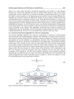
(1) Spread Information (2) Relational Design Information
Figure 1: Image of spread information and relational design information
To consider the methods of transmitting information, we classify the design information as follows.
1) Model design information
a) Single design information (EX: weight limitation, volume limitation etc.)
b) Relational design information (EX: boundary information etc.)
2) Element design information included in the model
a) Single design information
Information should spread to newly generated elements by using the initial element. For
example, surface roughness defined to the initial axis element should be migrated to the newly
generated face when a rotated solid is generated by specifying the initial axis. In this case, there
are two patterns; one is spreading to all generated faces unconditionally, or to specify the
generated face to spread. Fig. 1-(1) shows an example.
106
Ch22-I044963.fm Page 106 Tuesday, August 1, 2006 3:32 PM
Ch22-I044963.fm Page 106 Tuesday, August 1, 2006 3:32 PM
106
b) Relational design information
For the case of geometric type change, the system should handle the capability to maintain the
members of groups. Where, relational design information consists of two groups in Fig. l-(2).
If parallelism is defined between two initial lines, the system should add the axis of the rotated
object as a group member when the rotated object is generated.
Consideration of fuzziness concerning positioning
We consider the two types of fuzzy positioning. One is to define rough position; this is a case to
possible to define the space in which it can exist. The other is to define relative position. Naturally,
there is a case to define both. In the proposed architecture, this is able to be defined as the relational
design information between a target model and space. The relative positioning between targets, it is

possible to define the big or small conditions as Fig2-(2). Fig. 2-(l) shows patterns of relative
conditions. To define several conditions for each coordinate, it is able to define the relative condition
between targets. Where, MinX means the minimum x-coordinate extent and MaxX means the
maximum x-coordinate extent.
< behavior definition> <name>Relative positioning </name>
< characteristic value of element editing method>
< group characteristic valuc> <group no>l </group no>
< characteristic value>MaxX</ characteristic value>
</ group characteristic value>
<comparison ope ><!CDATA|=<||x/compariso n
ope»
< group characteristic value> <group no>2</group no>
< characteristic value>MaxX</ characteristic value>
</ group characteristic value>
</ characteristic value of element editing method>
Figure 2: Patterns of relative position for interval and example of x-coordinate behavior definition
Consideration for expression of function
In this section, it is discussed about two functional representations.
1) Behavior
Under certain situations, it is thought about the function as behavior. For example, a motor which
generates a rotary motion, the influence of the rotary motion has on the models is not considered. This
idea thinks an importance of potential influence. Thus, it is able to handle this design information as a
single design information in the proposed architecture.
2) Action
This idea is that the function is some action for the targets. Therefore, it is possible to express by using
a verb and object. Then, it is able to handle this design information as relational design information.
Thus,
the propose architecture can express the function as a behavior or an action.
Consideration for expression of space
Existence space where object can exist is a typical example of space. The space can be greatly

classified into two types. One is the space which relates directly to the arrangement of an object,
existence space or the space according to movement of object, etc. The other type is pure space,
which itself has some design meaning, midair or a cavity in a target, a closed space surrounded by
several object and the space which shows flows etc
1) Space which relates directly to object with substance (Territory of geostationary and movement)
2) Space which is defined by surrounding it with several objects (The existence space of a fluid or
107
Ch22-I044963.fm Page 107 Tuesday, August 1, 2006 3:32 PM
Ch22-I044963.fm Page 107 Tuesday, August 1, 2006 3:32 PM
107
gas)
This is a pure space and is defined as a space including a specified point.
Thus,
both spaces are defined as a geometrical data. Therefore it is possible handle the space as a
target for attaching design information and the intention. The expression of the space which relates
directly to an object with substance is possible to treat the relational design information between the
target object, space and pure space is possible to treat the single design information as a point.
Fig.3-
(1) shows the space which shows tracks of object and Fig. 3-(2) shows a case of personal computer
and shows the space of air flow for cooling and Fig. 4 shows a example of pure space.
Hr • ~' "
P
lp
'*
t
^If
••lib"
-m*
1
1

(1) Tracking space (2) The space of air flow for cooling
Figure 3: Example of the space
Figure 4: Example of closed space
Moreover, to handle the air flow and a closed space accentually, it is necessary for the mechanism to
evaluate the space conditions, opening, closing or penetrating. For example, Fig. 4 shows a
suspension part and the space in which oil is filled. The capability to check the open or closed state of
this space is very important. It explains the judgment of the opening and closing space, as follows. For
simplicity, all of the parts are solid models.
Proposition: Determination the open or closed state of space
Judgment
First, we show several definitions
P : Point included in space to be judged , Bi (i=l,2,,,,n): Parts which compose the suspension
H : The minimum hexahedron including the all parts
He : The hexahedron which expands +e (>0) for each coordinate. BD(He) : Boundary set of He
Then, if we take the differences of all parts from He, in general it becomes several solids.
U
Sj = He - [J Bi
i
- I i - i
So,
point P is included in Sk for some k. At that time, we can judge the state of space including
point P as follows.
Tf b e Sk for some b e BD(He)
108
Ch22-I044963.fm Page 108 Tuesday, August 1, 2006 3:32 PM
Ch22-I044963.fm Page 108 Tuesday, August 1, 2006 3:32 PM
108
Then the specified space is opened, else the specified space is closed
End of judgment.
5. SUMMARIES AND CONCLUSION

In this paper, we proposed the important items at the upstream design stage and shows the expressions
based on the principal architecture and its extension. Thus, proposed architecture is extensible and can
transmit the design information and intention from the upstream to the downstream design stage. In
the upstream design stage, shape and positioning are very simple or vague. To handle this information,
we introduced the migratory information and proposed the expression of relative positioning and
functions. To handle this information and to transmit this information to the downstream design stage
is very effective to achieve the main design intention.
Moreover, it is proposed the treatment of spaces, especially the classification of the space and the
judgment of the space state. In the actual design process, it is very important to transmit design
information and intention from the upstream design stage to the detailed design stage. This is very
important and effective not only the efficiency (reduction of design error or redo), but also for
achieving the product concept and the main customer requirements.
The proposed architecture is extensible and accurate to transmit the design information. This
architecture is one of the effective approaches to support the design process with the design
information and intention.
REFERENCES
[I] Yoshikawa.H and Tomiyama.T (1989,1990):,Intelligent CAD, Asakura-syoten, Tokyo Japan
[2] Pahl.G and Beitz.W(l 988), Engineering Design Systematic Approach, Springer-Verlag, Berlin
[3] Arai.E, Okada.K, and Iwata.K(1991), Intention Modeling System of Product Designers in
Conceptual Design Phase, Manufacturing Systems, Vol.20, No.4, pp.325-333
[4] Umeda.Y, Ishii.M, Yoshioka.M, Shimomura.Y, and Tomiyama.T(1996), Supporting Conceptual
Design Based on the Function- Behavior- State Modeler, Artificial Intelligence for Engineering
Design, Analysis, and Manufacturing, Vol.10, No.4, pp.275-288
[5] Stone.R.B, Wood.K.L(2000), Development of a Functional Basis for Design, Journal of
Mechanical Design, and Vol.122, pp359-370
[6] Arai.E, Akasaka.H, Wakamatsu.H, and Shirase.K(2000), Description Model of Designers'
Intention in CAD System and Application for Redesign Process, JSME Int. J. Series C, Vol.43,
No.
1, pp. 177-182
[7] Chakrabarti.A (ed.)(2000), Engineering Design Synthesis - Understanding, Approaches, and Tools,

Springer-Verlag, London
[8] Liu.J, Arai.E and Igoshi.M(1995), Qualitative Kinematic Simulation for Verification of Function
of Mechanical products, Trans JSME(C),
Vol61 ,
No585, pp.2159-2166, Japanese
[9] Liu.J, Amnuay.S, Arai.E and Igoshi.M(1996), Qualitative Solid Modelling : 1st Report,
Qualitative Solid Models and Their Organization, Trans JAME(C)), Vol62, No599, pp.2897-2904,
Japanese
[10] Takeuchi.K, Tsumaya.A, Wakamatsu.H, Shirase.Kand Arai.E(2003), Expression and Integrated
Model for Transmission of Design Information and Intention, Proc. 6th Japan-France Congress
on Mechatronic, pp83-88
[II] Takeuchi.K, Tsumaya.A, Wakamatsu.H and Arai.E(2004), Extensibility for Integrated Model of
Geometrical and Intetional Information, JUSFA 2004, JL013
109
Ch23-I044963.fm Page 109 Tuesday, August 1, 2006 9:09 PM
Ch23-I044963.fm Page 109 Tuesday, August 1, 2006 9:09 PM
109
DETECTION OF UNCUT REGIONS IN POCKET MACHINING
Manseung Seo
1
, Haeryung Kim
1
and Masahiko Onosato
2
1
Department of Robot System Engineering, College of Engineering, Tongmyong University,
535 Yongdang-dong, Nam-gu, Busan
608-711 ,
Korea
Graduate School of Information Science and Technology, Hokkaido University,

Kita-14, Nishi-9, Kita-ku, Sapporo, Hokkaido 060-0814, Japan
ABSTRACT
Upon realization of the fact that uncut regions exist if there is an intersection between a previous tool
envelope and a current tool envelope, this study is initiated. As a key concept, the Tool envelope Loop
Entity (TLE) is devised to treat every trajectory made by the tool radius as an ordinary offset loop. The
TLE concept enables the offset curve generation method to be extended further as a distinctive method
in which uncut region detection is done through an identical way of offsetting. To ensure the method
works, a prototype system is implemented and evaluated with the tool path generation obviating uncut
regions. The result verifies that the proposed method fulfils technological requirements for uncut free
pocketing.
KEYWORDS
Pocket, Offset, Offset Loops, Uncut Region, Clean up Curve, Tool Path.
INTRODUCTION
It is not easy to find an efficient method for tool path generation free from uncut regions. In the
literature, to solve uncut problems, Held et al. (1994) employed a specific adjustment on successive
offset distance through the Voronoi diagram approach and Park & Choi (2001) took local care on tool
trajectories through the pair-wise intersection approach. Recently, for offset curve generation, Seo et al.
(2004) proposed the Offset-loop Dissection Method (ODM) based on the Offset Loop Entity (OLE)
concept, which enables the method to be implemented easily into the system at any condition,
regardless of the number of offsets, the number of intersections, and even the number of islands.
Recognizing the robustness and flexibility of the ODM and realizing the fact that uncut regions exist if
there is an intersection between a previous tool envelope and a current tool envelope, we extend the
ODM to uncut region detection. For the adoption of the ODM, we define the Tool envelope Loop
110
Ch23-I044963.fm Page 110 Tuesday, August 1, 2006 9:09 PM
Ch23-I044963.fm Page 110 Tuesday, August 1, 2006 9:09 PM
110
Entity (TLE), i.e., the trajectory made by the tool radius, as a key concept corresponding to the OLE to
treat every tool envelope as an ordinary offset loop. The uncut region detection method, namely the
extended ODM is proposed. The conspicuous feature of the devised method is that uncut regions are

detected in an identical way of offsetting and the clean up curves are treated as ordinary offset loops.
Through this study, the problem of obviating uncut regions is resolved.
GENERATION OF OFFSET CURVE FOR POCKETING
To focus the present study on the detection of uncut regions, offset curve generation for pocketing
without or with islands is briefly discussed through an illustrated example shown in Fig.l. The
boundary of the pocket is defined as the Contour curve Entity (CE) and the sequential linkage of the
CEs is defined as the Contour Loop Entity (CLE) as shown in Fig.l(a), by assuming that a CLE is
constructed only with lines and circular arcs. Imagining that a circle with a radius that equals the offset
distance is rolling on the CE, the trajectory of the center of the circle is defined as the Offset curve
Entity (OE), and the sequential linkage of OEs is defined as the inborn OLE as shown in Fig.
1
(b). In
pocket machining, there is a strong possibility that the inborn OLE is formed into an open loop having
local and global self-intersections that result in undesirable cuts. The local OLE reconstruction is
performed inserting additive OEs or by dissecting intersections in two adjacent OEs to create one
crude OLE and to discard four open OLEs as shown in Fig. l(c). However, the crude OLE is
intersected globally by itself at three points as shown in Fig.l(d). Detecting an intersection and
applying a dissection on the crude OLE, the OLE is decomposed into one simple OLE and one crude
OLE. By the second dissection, the OLE is decomposed into one simple OLE and one crude OLE. By
the third dissection, the OLE is decomposed into two simple OLEs. Finally, all OLEs become simple
OLEs as shown in Fig.l(e). The simple OLE obtained by the global OLE reconstruction may still not
be appropriate as an offset curve for machining. The characteristics of OLE, i.e., closeness and
orientation, need to be examined to confirm the validity of OLE for continuity and proper direction of
the tool path. Fixing the orientation of a CLE to be counterclockwise, two OLEs are selected as valid
OLEs,
since they are completely closed and counterclockwise. Then, the valid OLEs in Fig.l(f) are
kept to play the role of an offset curve for pocketing and the role of CLEs in the next offsetting turn.
One of the salient features of the ODM is the applicability. The offset curve generation method for one
OLE works as the method for multiple OLEs. To ensure the merits, the ODM is applied to the
generation of an offset curve for a pocket with islands, by shifting the object of intersection detection,

dissection, and validation, from one OLE to multiple OLEs. Using an illustrated example of offset
curve generation for a pocket with an island, the ODM is evaluated. Figure l(g) shows the CLEs from
one pocket and one island in dotted line, and two simple pocket OLEs and one simple island OLE in
solid lines. At an intersection, a pocket OLE and an island OLE are dissected, and reconnected into
one combined OLE conserving orientations and vice versa. Then, applying a dissection one more time
at the other intersection and reconnecting again, one combined OLE is decomposed into two combined
OLEs as shown in Fig.l(h). Performing OLE validation with the rule that the characteristic of the
pocket OLE is transferred to the combined OLE when a pocket OLE and an island OLE are combined
into an OLE, two valid OLEs are kept to play the role of offset curves for pocketing and the role of
CLEs in the next offsetting turn as shown in Fig.
1
(i). Thus, the ODM works for a pocket with islands.
DETECTION OF UNCUT REGIONS
Uncut regions appear mainly on two occasions. The first is due to the improper selection of tool
diameter for pocket boundary. There is no way to avoid this kind of uncut, unless the other tool is
selected. The second is due to the complexity of pocket geometry under the offset distance properly
111
Ch23-I044963.fm Page 111 Tuesday, August 1, 2006 9:09 PM
Ch23-I044963.fm Page 111 Tuesday, August 1, 2006 9:09 PM
111
fixed for tool diameter and high speed milling. It is avoidable, and is still worthwhile to develop a
better way of obviation. Upon realization of the fact that uncut regions exist if there is an intersection
between a previous tool envelope and a current tool envelope, the ODM is extended to the uncut
region detection and clean up curve generation based on the TLE concept, which enables the ODM to
be easily applied to uncut region detection. The method, namely the extended ODM, is proposed by
shifting the object of ODM from OLEs to TLEs.
To verify the extended ODM, the entire process of uncut region detection and clean up curve
generation is evaluated through an illustrated example shown in Fig.2. Figure 2(a) shows the previous
[(n-l)
th

] tool path, the current [(n)
th
] tool path, the inward trajectory made by the previous tool path
(previous TLE), and the outward trajectory made by the current tool path (current TLE). By taking a
glance at Fig.2(a), we easily notice that the uncut region exists if there is an intersection between
previous TLE and current TLE. Moreover, by imaging that the previous tool path to be like a pocket
CLE and the current tool path to be like an island CLE, the previous TLE may be considered as a
pocket OLE and current TLE may be considered as an island OLE, and then, we could see that those
exactly match as shown in Fig.2(b). Therefore, we just need to carry out the ODM to detect the uncut
regions upon OLE/TLE concepts. After the previous/current TLEs construction, the TLE
reconstruction is processed as we did in the offset curve generation of the pocket with one island in
Fig.l. Then, non-intersecting simple TLEs are obtained as shown in Fig.2(c). Performing TLE
validation with the rule that the characteristic of the previous TLE is transferred to the combined TLE
when a previous TLE and a current TLE are composed into a TLE, four simple TLEs with clockwise
orientation are discarded. Finally, four valid TLEs corresponding to the boundaries of uncut regions
are kept to play the role of the clean up curve. The clean up curves are then appended to current valid
OLEs taking the shortest line segment for the construction of an uncut free tool path, as shown in
Fig.2(d). Here, we may conclude that the extended ODM is flexible and robust enough to generate
offset curves for uncut free pocket machining with islands.
(a) Boundary of pocket
(d) OLE with glob;
(b) Local and glol
(c) OLE without intersection
(c) Dissection at
(g) Simple OLEs from pocket and island (h) Combined OLLs without intersection
(i) Offset curve for pocket with island
Figure 1: Offset curve generation procedures for a pocket with an island
112
Ch23-I044963.fm Page 112 Tuesday, August 1, 2006 9:09 PM
Ch23-I044963.fm Page 112 Tuesday, August 1, 2006 9:09 PM

112
RESULTS AND DISCUSSION
In order to verify the salient features of the extended ODM, a prototype system is implemented using
C language and Open GL graphic library. The screen image of an uncut free tool path obtained from
the implemented system is shown in
Fig.3.
The uncut regions are detected and then attached to the
offset contours. The result of the implemented system verifies that the devised method is robust
enough to generate uncut free tool paths.
CONCLUSIONS
In this study, we proposed the extended ODM for uncut free tool path generation. The OLE/TLE
concept enables the ODM to possess robustness and flexibility. The distinctiveness comes from the
facts:
1) The entire procedure is systematically integrated using the OLE/TLE, 2) Every procedure
deals only with the OLE/TLE, and 3) Each procedure is designed based on the OLE/TLE. Thus,
through this study the problem obviating uncut regions is resolved and the high speed milling becomes
feasible.
REFERENCES
Held M., Lukacs G. and Andor L. (1994) Pocket machining base on contour-parallel tool paths
generation by means of proximity maps, Computer Aided Design, 26:3, 189-203.
Park S. and Choi, B. (2001). Uncut free pocketing tool-paths generation using pair-wise offset
algorithm, Computer Aided Design, 33:10, 739-746.
Seo M., Kim H. and Onosato M. (2005) Systematic approach to contour-parallel tool path
generation of 2.5-D pocket with islands, Computer-Aided Design and Applications, 2:1, 213-222.
Prcwoii
s
[(n- 1 )
L
"J too l pul h Curren t [(u)'
1

'] tool path Pocke t
CI,
Y
r
T
T
1
Pocke t OL E Islan d
OLE
(b) Pocket/islan d CT.E s
ami
OT.E s
*
(d) Clea n
up
pat h appende d
lo
curren t
OLF.
Figure 2: Uncut region detection procedures Figure 3: Uncut free tool path
113
Ch24-I044963.fm Page 113 Monday, August 7, 2006 11:27 AM
Ch24-I044963.fm Page 113 Monday, August 7,2006 11:27 AM
113
FLEXIBLE PROCESS PLANNING SYSTEM CONSIDERING DESIGN
INTENTIONS AND DISTURBANCE IN PRODUCTION PROCESS
G Han
1
M. Koike
2

H. Wakamatsu
1
A. Tsumaya
1
E Araf andK. Shirase
3
1
Department of Manufacturing Science, Graduate School of Eng., Osaka University
2-1 Yamadaoka, Suite, Osaka, 565-0871, Japan
2
Department of Systems Design, College of Industrial Technology
1-27-1
Nishikoya, Amagasaki, Hyogo, 661-0047, Japan
3
Department of Mechanical Engineering, Faculty of
Eng.
Kobe University
1-1 Rokkodai,Nada, Kobe, Hyogo, 657-0013, Japan
ABSTRACT
Improvement of machining process planning is an effective way to reduce manufacturing time and cost, and to
achieve the desirable functions which are described by designers. This paper proposes a machining process
planning system which can flexibly perform process planning, considering design intentions and dealing with
disturbances in the manufacturing process by choosing the optimum plans from multiple candidates. The core of
the mechanism consists of (l)Extraction of Total Removal Volume(TRV), (2)Decomposition of the TRV into
Minimum Convex Polyhedrons (MCP) (3)Recomposition of MCPs into feasible manufacturing features
sets(MF set), (4)Recognition of manufacturing feature(MF), (5)Determination of machining sequences by
considering various constraints, and (6)Comparison of each candidate containing a certain MF set and
machining sequence to obtain the most optimum plan. All the functions are realized and implemented on DLL
format compiled in Visual C++ and SolidWorks API.
KEYWORDS

Computer Aided Process Planning, Manufacturing Feature, Machining Sequencing
1.
INTRODUCTION
Process planning plays a key role in modem manufacturing. And it provides the functions which translate
114
R
aw stock Finished
p
ar
t
Extraction of TRV
Decomposition of TRV to MCPs
Generation of desirable MFs
Recomposition of remained MCPs
Determination of Machining
Evaluation of the Machining time
Constraint
Conditions
Constraint
Conditions
Ch24-I044963.fm Page 114 Monday, August 7, 2006 11:27 AM
Ch24-I044963.fm Page 114 Monday, August 7,2006 11:27 AM
114
designers' intentions and finished parts' specifications into technologically feasible plans describing how to
manufacture a functional part efficiently and precisely. The task of automatically generating a process plan from a
solid model representation of a part is normally subdivided into several activities such as: selection of the
machining operations and so on. A process plan should primarily consist of a Manufacturing feature (MF) set
which describes the most suitable removal volume set and a machining sequence which are considered optimum
for the design intentions and the current manufacturing conditions. Most of current manufacturing systems
perform fixed process planning which often leads to provide "fixed plans" for production. Those plans are only

applicable in the situation where no errors and disturbances are found during the manufacturing process and no
alterations are made to facilities in workshop [1]. Moreover, in some cases, because manufacturing features
interpretations are predefined in a fixed way, only small number of plans can be generated as candidates. In
addition, those outputted process plans are usually proven not the most efficient and precise for manufacturing.
Because a great deal of useful embedded information in the part model is ignored, the determined sequences often
fail to satisfy the desirable functions. As a result, the flexibility of process planning becomes an essential and
effective way to create more candidates for resolving this problem. To realize the flexibility, our proposed system
generates more functionally and technically satisfactory candidates. Finally, the most optimum process plan will
be chosen from the candidates by comparing machining time of each plan.
Raw stock
" 1
Finished part
r
Extraction of TRV
Decomposition of TRV to MCPs
Constraint
Conditions
nditions
Generation of desirable MFs
Recomposition of remained MCPs
Constraint
Conditions
nditions
Determination of Machining
Evaluation of the Machining time
Figure 1: Core parts of the system
2.
SYSTEM ARCHITECTURE
This system provides functions of generating one or more candidates of MF set to suit variable machining
circumstances, sequencing the MFs and determining the best process plan which can realize the designed part,

respecting the desired quality at high efficiency. The overall goal of this flexible process planning system is
obtained through the following main steps shown in Fig.l The manufacturing feature recognition is executed
based on judging the number of the open faces of the feature, by retrieving and modifying the familiar cases from
database, case-based reasoning decides machining conditions including tools, cutting conditions, tool path and so
115
(a) (b)
(c)
Face 1
Face 2
Ch24-I044963.fm Page 115 Monday, August 7, 2006 11:27 AM
Ch24-I044963.fm Page 115 Monday, August 7,2006 11:27 AM
115
on for individual features [2].
(b)
Face1
(c)
Figure2: Extraction of TRV (a) raw stock (b) resigned product (c) extracted TRV
3 FEATURE INTERPRETATIONS
This system offers multiple feature interpretations, which are represented in the form of MF st through the
following steps:
3.1 Extraction of TRV
Process planning starts with the extraction of the removal area which is mainly composed by the planes and
cylindrical surfaces in this system. The removal area is computed through difference between the raw stock and
finished part. The volume generated in this subtraction process is named Total Removal Volume (TRV). Some
parts with complex shapes usually offer TRV composed of more than one removal volume, these volumes are
defined as SRV (Sub Removal Volumes) which will be handled respectively. Fig.2 shows an example of the
extraction of TRV composed of four SRVs, and one of the iaces (Face 1) in the part model and its corresponding
face (Face 2) in TRV share the same attributed infbrmatioa
3.2 Decomposition ofTRVinto MCPs
For generating enough sets of machinable MFs to cope with diversified facility circumstances and disturbances

found in workplace, each SRV will be decomposed into Minimum Convex Polyhedrons (MCP) which can be
recomposed into multiple sets of manufacturing features in the next steps. In this system, decomposition is
performed by the cutting planes that are generated referring to all the planar faces in each SRV. Every planar face
which belongs to SRV is extended enough to split SRV (as in Fig.3). Cylindrical faces will not be considered to
create cutting faces. Then system randomly selects one cutting face to bisect SRV and if the SRV is intersected
with this cutting face, several new volumes which have one or more created faces will be generated. At the same
time,
some faces which are attributed with constraints information in the SRV are split into several small iaces in
separate MCPs. The information is to be inherited from parent laces to new-created faces for delivering the
demands information about part manufacturing to later steps. Then the procedures above repeats itself by utilizing
other cutting facesto cut all cuttable new-born volumes and original SRVs until all the cutting faces are used The
example about decomposition of the former TRV is shown in the Fig.3 (b).
116
(a)
(b)
(a) (b)
Ch24-I044963.fm Page 116 Monday, August 7, 2006 11:27 AM
Ch24-I044963.fm Page 116 Monday, August 7,2006 11:27 AM
116
(a) (b)
Figure 3: TRV decomposed into Minimum Convex
!> •
(a)
(b)
Figure 4: Attributed MCPs and generated MFs
3.3 Generation of the desirable MFs
Manufacturing feature each of which is removed with a single machining operation is a combination of a number
of MCPs. Because the tool condition and cutting conditions keep unchanged without tool exchange, machining
MCPs attributed with the same demand information as one MF can guarantee the high quality. The MFs(MF set)
which can actualize the requirements are generated by recomposing the demand-attributed MCPs. System gathers

the MCPs which are demanded by the same description, and combine them into one machinable MF. For example,
two cylindrical MCPs with same concentricity and four MCPs sharing the same face which is required by the
same surface finish are shown in Fig.4 (a), and the desirable features generated are shown in (b) respectively.
1 level Z level
-•fv;
Figure 5: MCPs in different levels
3.4 Recomposition of remained MCPs to MF sets
In this step, the uncombined MCPs without any demand attribution are recomposed to obtain several sets of MFs.
Merging these MCPs in different ways leads to different MF sets. MCPs that generated through decomposition are
117
Ch24-I044963.fm Page 117 Monday, August 7, 2006 11:27 AM
Ch24-I044963.fm Page 117 Monday, August 7,2006 11:27 AM
CD 0.1
117
grouped into distinguished levels according to their geometrical position. MCPs whose top Z axis-perpendicular
faces share the same Z coordinate value are defined as same level MCPs. An example of remained MCPs, which
are classified into 3 levels are illustrated in
Fig.5.
Because tool properties such as length and strength restrict the
sizes of machinable MFs, recomposition is to be executed level by level to avoiding creating MFs which are
machinably unavailable in TAD (Tool Approach Direction).
Z level 1
Z level 2
Z level 3
(b) (
c
) Figure 7: Determination of the shortest machining time of aMF set
(a) SRV with one lace demanded by the same constraint of flatness which is valued 0.1
(b) Three MFs ought to be machined continually
(c) Two MFs ought to be machined continually

Figure 6: Determination of machining sequence
4 MACHINING SEQUENCE
One of the important and difficult activities in process planning is the determination of sequence which causes
high-quality parts to be produced efficiently. For producing the part here are more than one set of features
available to be chosen Even tor one of such sets of MFs, there are many ways to sequence these features for
machining. But the utilization of all the possible MF set as removal area descriptions to determine the optimum
process plans is rather time-consuming because the huge number of alternatives will overload the system. The
constraints h workplace environment and design intentions are considered to eliminate the improper MF sets
before they are further used for process planning, Because the majority of current systems focus too much on
creating sequences based on part geometry, and fail to utilize other information which describes the designers'
intentions, The final sequence plans often dissatisfy the requirement of qualities and functions, or are relatively
time-consuming. Based on the constraint rules, which are developed and applied, the constraints obtained from the
designer's intentions or the factory environment will be used to resolve this problem. F)ue to tools' restrictions in
length and hardness, machining the MFs that are too large in TAD should be avoided. Therefore in this system
sequencing is executed in each level. The solution of one MF set begins with recreating ID numbers to identify
remained MFs in one level and sorting all these MFs in this level to generate all possible machining sequences as
candidates. The vast number of feasible sequences will become evident through this mean. Without consideration
of the constraints in manufacturing, it would be possible 6r a level composed of N manufacturing features to be
processed from one of N factorial sequences. An obvious choice would be to represent a sequence as a string,
whose elements are ID of features in a level of this MF set But in reality this number of the alternatives is reduced
by the feasible constraints. Appropriate sequences of each level are extracted from these choices. All the feasible
sequences are checked based on geometry constraints, tolerance constraints, and quality constraints. Finally only
the satisfactory sequences are picked out for machining time evaluation. Main constraints taken into
considerations in this system are: Cylindricity, flatness, dimension tolerance, concentricity, surface finish. The MFs
118
Ch24-I044963.fm Page 118 Monday, August 7, 2006 11:27 AM
Ch24-I044963.fm Page 118 Monday, August 7,2006 11:27 AM
118
that satisfy the same constraints are to be continually machined. So the strings described by the correctly sorted
numbers, whose order represents machining sequence are delivered to the next step. Then the decoding process is

applied, translating each code into the string of the features. At last, a number of process plans which comprised of
a set of feature interpretation and its machining sequence are provided for optimum plan determination. A simple
example about two MF sets desired to be machined continually are shown in Fig.6.
5. OPTIMUM PROCESS PLAN
Because the determination of feature interpretation and sequencing are based on the requirements in qualities and
functions, in this system machining time is used as the major criterion in effectiveness evaluation to decide optimal
or near-optimal plan. The factors that affect the machining time involve (a) cutting condition generated by
case-base reasoning in this system, (b) path length estimated by considering the sizes and machining sequences of
the MFs, (c) the effect of surface quality. The machining time consists of cutting time, tools exchanging time and
the time cost when tools travel between manufacturing features. The total machining time in a level of a MF set is
calculated with the following equation.
-*- level -* • i'L'*jtiiFe -*- too! cxch-jtige -* • Vi&tejf
Where T(level) is the time cost in the process of machining all the MFs of this level. T(Feature) is the time spent
on removing MFs, T (toolexchange) is time for exchanging tools, and T(travel) stands for the time used in
traveling the tools between MFs. Until this step one MF set still possesses more than one appropriate machining
sequence each of which cause different machining time. The calculated machining times of every level in one MF
set are aligned as Fig. 7. The nodes in the figure show the machining time of every sequenced level in every MF
set, the two numbers in the node indicate the level number and the machining sequence number respectively, the
time which are spent on traveling tools between levels are taken into account as well. The path with the minimum
time in the tree means the most efficient machining flow of this MF set. Compared with other MF sets, the
corresponding process plan with the shortest machining time is decided as optimum plan for manufacturing this
part.
6. CONCLUSION
By taking into account the designer's intentions and making use of the functional and technical constraints, the
system proposed in this paper can provide the most optimum process plan for manufacturing the designed part.
REFERENCES
[1] Nagafune N., Kato Y, and Matsumoto T.(1998). Flexible Process Planning based on Flexible Machining
Features. JSME journal 75,127-128.
[2] Shirase K., Nagano T, Wakamatsu
FL,

and Arai E.(2000). Automatic Selection of Cutting Conditions Based on
Case-Based Reasoning. Proceedings of 2000 International Conference on Advanced Manufacturing Systems
and Manufacturing Automation, 524-528
119
Ch25-I044963.fm Page 119 Tuesday, August 1, 2006 3:36 PM
Ch25-I044963.fm Page 119 Tuesday, August 1, 2006 3:36 PM
119
A STUDY ON CALCULATION METHODS OF ENVIRONMENTAL
BURDEN FOR NC PROGRAM DIAGNOSIS
H. Narita
1
, T. Norihisa
2
, L. Y. Chen
1
, H. Fujimoto
1
and T. Hasebe
2
'Graduate School of Engineering, Nagoya Institute of Technology,
Gokiso-cho, Showa-ku, Nagoya, Aichi, 466-8555, Japan
2
OKUMA Corporation,
5-25-1,
Shimokoguchi, Oguchi-cho, Niwa-gun, Aichi, 480-0193, Japan
ABSTRACT
Some activities for environmental protection have been tried to reduce environmental burdens in a lot
of fields. Manufacturing field is also required to reduce them. Hence, prediction system of
environmental burden for machining operation is proposed based on LCA (Life Cycle Assessment)
policy. This system can calculate environmental burden (equivalent CO2 emission) due to the electric

consumption of a machine tool, the cutting tools status, the coolant quantity, the lubricant oil quantity
and the metal chips, and provide the information of the accurate environmental burden of the
machining process by considering some activities related to the machine tool operations. In this paper,
the development status of prediction system is described. As a case study, two NC programs that
manufacture simple shape are also evaluated to show the feasibility of it.
KEYWORDS
Environmental burden, Life Cycle Assessment, Production cost, Machine tool operation, Virtual
machining, NC program diagnosis
INTRODUCTION
Manufacturing technologies pursuing the sustainable development are required due to the evident
environmental impacts like global warming, ozone layer depletion and acidification, so manufacturing
system has to be reassessed from the view point of environmental protection. Hence an accurate
evaluation system of environmental impacts for manufacturing is required. But it is difficult to
evaluate environmental impacts because we can not recognize them. In this research, a prediction
system of the environmental burden for a machining operation is proposed based on LCA (Life Cycle
Assessment) (SETAC, 1993) policy for future manufacturing system. This kind of system will enable
engineers to decide the machining strategies, to generate the production scheduling and to evaluate the
120
Ch25-I044963.fm Page 120 Tuesday, August 1, 2006 3:36 PM
Ch25-I044963.fm Page 120 Tuesday, August 1, 2006 3:36 PM
120
new manufacturing technologies with considering
the
environmental impact.
In
this paper,
a
conceptual architecture
and a
system design

of the
environmental burden calculation system
are
introduced first. Then, calculation algorithm
of
the environmental burden
due to the
machine tool
operation
is
proposed and
the
feasibility
of it is
shown through
a
case study. Furthermore, using
the
cost data, NC programs are evaluated from the view points
of
the global warming and the production
costs,
and low environmental burden and low cost machining operations are discussed
SYSTEM OVERVIEW
Figure
1
shows an overview
of
the proposed evaluation system
of

environmental burden
for
machining
operation.
A
work piece information, some cutting tools information and
an
NC program are input
to
the analysis model, the activities related
to
the machine tool operation and the machining process
are
estimated. Then,
the
electric consumption
of a
machine tool,
the
cutting tool status (tool wear),
the
coolant quantity,
the
lubrican t quantity, the metal chip quantity and other factors
are
evaluated. Here,
other factors correspond
to the
electric consumption
of

light,
the air
conditioning
and so on.
Using
these estimated information and the emission intensities data and the resource data, the environmental
burden
is
calculated, when
a
product
is
manufactured.
The
emission intensities data means
the
parameters required
for the
calculation
of
environmental burden. These emission intensities
are
prepared according
to
impact category such
as
the global warming,
the
ozone layer depilation and
so

on. The resource data also means the machine tool specification data, cutting tool parameter, etc.
for
the estimation
of
machining process. This system can calculate
the
environmenta l burden
in
various
cutting conditions, because the machining process
is
evaluated properly. This
is a
novel feature
of
the
system.
NC program
Database
Machine tool Machining proces
Quantity olcooUml and lubric
OuaiiLlvofmolaldiips
Envin nmental burd
inoak.
lator
•)
Figure
1:
Processing flow
of

the prediction system developed
in
this research
CALCULATION ALOGORITHM
The total environmental burden
is
calculated
by
equation
(1). The
calculation algorithm
of
environmental burden
is
the following.
Pe = Ee + Ce
+ We +
]T (7e,.)+ CHe + OTe
i=\
Pe: EB
of
machining operation [kg-GAS]
Ce: EB
of
coolant [kg-GAS]
Te: EB
of
cutting tool [kg-GAS]
OTe: EB
of

other factors [kg- GAS]
(1)
Ee: EB
of
machin e tool component [kg-GAS]
We: EB
of
lubricant oil [kg-GAS]
CHe: EB
of
metal chip [kg- GAS]
N: Number
of
tool used
in
an NC program
EB:
Environmental burden
121
Ch25-I044963.fm Page 121 Tuesday, August 1, 2006 3:36 PM
Ch25-I044963.fm Page
121
Tuesday,
August
1,
2006
3:36 PM
121
Electri c consumptio n of machin e tool (Ee)
The environmenta l burden due to the machin e tool electri c consumptio n is expresse d by equatio n (2).

In equatio n (2), the electri c consumptio n of the servo motor s and the spindl e moto r is varied
dynamicall y accordin g to the machinin g process , so the electri c consumptio n of these motor s are
calculate d with considerin g the table weight , the frictio n coefficient s of the slide way, the ball screw
lead, the transmissibilit y of the ball screw , the axial frictio n torque , the cuttin g force and the cuttin g
torque. Here , these are also predicte d by cutting proces s mode l (Narita , et. al, 2002) . This cuttin g
process mode l concep t can be applie d to squar e end millin g operation , ball end millin g operation ,
turning operatio n and so on. Using these models , variou s cutting processe s can be evaluated .
Ee = kx(SME+ SPE +SCE+CME +CPE+TCE1+TCE2+ATCE+MGE+VAE) (2 )
k: CO2 emissio n intensit y of electricit y [kg-GAS/kWh ]
SME: EC of servo motor s [kWh ] SPE: EC of spindl e motor [kWh ]
SCE: EC of coolin g system of spindl e [kWh ] CME: EC of compresso r [kWh]
CPE: EC of coolan t pump [kWh] TCE1: EC of lift up chip conveyo r [kWh ]
TCE2: EC of chip conveyo r in machin e tool [kWh ] ATCE: EC of ATC [kWh ]
MGE: EC of tool magazin e moto r [kWh] VAE: Vampir e energy of machin e tool [kWh ]
EC:
Electri c consumptio n
Coolan t (Ce)
There are two types cuttin g fluid, so two equation s are propose d for Ce evaluation . First , the water -
miscibl e cuttin g fluid is explained . The coolan t is generall y used to enhanc e the machinin g
performance , and circulate d in a machin e tool by a coolan t pump until the coolan t is updated . During
the period , some coolant s are eliminate d due to the adhesio n to the metal chips , so the coolan t is
supplie d for the compensation . The dilutio n fluid (water ) is also reduce d due to the vapor. So, the
equatio n (3) is adapte d to calculat e the environmenta l burden . Second , the water-insolubl e cuttin g
fluid is explained . In this case, the discharg e rate is an importan t factor . Hence , the equatio n (4) is
applied .
Ce
{(CPe + CDe)x(CC + AC)+fVAex(lVAQ+ Al¥AQ)}
(3 )
CUT: Coolan t usage time in an NC progra m [s] CL: Mean interva l of coolan t update [s]
CPe: EB of cuttin g fluid productio n [kg-GAS/L ] CDe: EB of cutting fluid disposa l [kg-GAS/L ]

CC: Initia l coolan t quantit y [L] AC: Additiona l supplemen t quantit y of coolan t [L]
WAe: EB of water distributio n [kg-GAS/L ] WAQ: Initial quantit y of water [L]
AWAQ: Additiona l supplemen t quantit y of water [L]
Ce=
CUTXCS
x(CPe
+
CDe) (4 )
3600x100 0
CS : Discharg e rate of cuttin g fluid [cc/h]
Lubrican t oil (LOe)
Lubrican t oil is mainl y used for spindl e and slide way, so two equation s are introduced . The minut e
amount s of oil are supplie d to the spindl e part in an interva l time. For the lubrican t of the slide way,
the certain amoun t of the oil is also supplie d by pump in an interva l time. So, the followin g equation s
are adapte d to calculat e the environmenta l burden due to lubrican t oil. These equation s can be adapte d
oil-air lubrican t and the grease lubricant .
LOe = Se + Le (5 )
122
Ch25-I044963.fm Page 122 Tuesday, August 1, 2006 3:36 PM
Ch25-I044963.fm Page
122
Tuesday, August
1,
2006 3:36 PM
122
Se =
^ x SV x
(SPe
+ SDe)
(6)

SI
LV(LP +
LD) (7)
Le
Se:
EB of
spindle lubricant
oil
[kg-GAS]
Le: EB of
slide
way
lubrican t
oil [kg- GAS]
SRT: Spindle runtime
in an
NC program
[s]
SV: Discharge rate
of
spindle lubricant
oil [L]
57:
Mean interval between discharges
[s]
SPe:
EB of
spindle lubricant
oil
production [kg-GAS/L]

SDe:
EB of
spindle lubricant
oil
disposal [kg-GAS/L]
LUT: Slide
way
runtime
in an NC
program
[s] LI:
Mean interval between supplies
[s]
LV: Lubricant
oil
quantity supplied
to
slide
way [L]
LPe:
EB of
slide
way
lubricant
oil
production [kg-GAS/L]
LDe:
EB of
slide
way

lubricant
oil
disposal [kg-GAS/L]
Cutting tool
(Te)
Cutting tools
are
managed from
the
view point
of
tool life.
So, the
tool life
is
compared with
the
machining time
to
calculate
the
environmental burden
in one
machining. Also,
the
cutting tools,
especially
for
solid
end

mill,
are
made
a
recovery
by
re-grinding,
so
these points
are
considered
to
construct environmental burden equation.
Te
= -^ ?x((TPe
+
TDe)x.TIV
+ RCNxRCe) (8)
MT: Machining time
[s]
TL: Tool life
[s]
TPe:
EB of
cutting tool production
[kg-
GAS /kg] TDe:
EB of
cutting tool disposal
[kg-

GAS
/kg]
TW: Tool weight
[kg]
RN: Total number
of
recovery
RCe:
EB of
tool recovery
[kg- GAS]
Metal chip {CHe)
Metal chips
are
recycled
to
material
by an
electric heating furnace. This materialization process
has to
be considered. This kind
of
equation
is
supposed
to
consider material kind,
but an
electrical intensity
of this kind

of
electric heating furnace
is
represent
by
kWh/t,
so the
equation constructed
in
this
research
is
calculated from
the
total metal chip weight.
CHe = (WPV-PV)xMDx
WDe
(9)
WPV: Work piece volume
[cm ]
PV: Product volume
[cm ]
MD: Material density
of
work piece [kg/cm
3
] WDe:
EB of
metal chip processing [kg-GAS/kg]
CASE STUDY

In order
to
show
the
feasibility
of
developed system,
a
case study
is
introduced. Then,
the
impact
category
is set to
global warming
to
calculate
the
environmental burden.
In
this research,
CO
2
, CH
4
and N2O
are
evaluated based
on

Japanese data, which
are
decided from environmental report, technical
report, home page
and
industrial table (Tokyo Waterworks, 2002, Tokyo Electric Power Company,
2002,
Nansai, 2002, Mizukami, 2002). Here,
CH
4
and
N2O emission
is
converted
to
equivalent
CO2
emission using
the
characterization factors
and
total
CO
2
emission
is
evaluated. Here,
the
global
warming potential (GWP)

of
100 years (IPCC, 1995)
is
used
for the
characterization factors.
The
other
emission matters related
to
global warming
are
ignored, because there
are no
emissions about
the
machining operations.
In
this case study, machine tool
is
MB-46VA (OKUMA Corp.), cutting tool
is
carbide square
end
mill with
2
flutes
and 30 deg.
helical angle
and

workpiece
is
medium carbon steel
(S50C).
The
simple product shown
in
Figure
2 is
evaluated.
123
Ch25-I044963.fm Page 123 Tuesday, August 1, 2006 3:36 PM
Ch25-I044963.fm Page 123 Tuesday, August 1, 2006 3:36 PM
123
The dry machining, the MQL machining and the Wet machining are evaluated in this case study. Here,
the life of cutting tool is assumed to be extended to 2 times of original one. The analyzed results are
shown in Figure 3. The equivalent CO2 emission of wet machining is largest and one of dry machining
is smallest in this comparison. Using this system, this kind of comparison can be carried out easily
from NC program. Here, the detailed discussion is tried based on the analyzed results. The portion of
electric consumption is highest in the all factors, obviously. This causes due to the peripheral devices
of machine tool. This factor is also proportional to machining time. That is to say the high speed
milling in dry machining method may be superior machining from the view point of CO2 emission
because of the short machining time, although detailed analysis will be required.
Dry L
0.00 20.00 40.00 60.00 80.00 100.00 120.00
Equivalent CO
2
emission g-CO
2
• Electric

snsumption
E3
Coolant
• Lubricant oil
Cutting tool
H Metal chip
Figure2: Product shape Figure 3: Analyzed environmental burden results
Also,
the equivalent CO2 emission of the MQL machining and the wet machining is larger than the dry
machining. As shown in the Figure 3, the equivalent CO2 emission of cutting tool is smaller due to the
mitigation of tool wear, but one of peripheral devices operated by coolant usage and one of coolant are
added and total one becomes larger. It is found, however, one of peripheral devices operated by
coolant usage is larger than one of coolant effect. Furthermore, equivalent CO2 emission of CH4 and
N2O is calculated using analyzed results of wet machining. These are related to environmental burden
of cutting fluid. Equivalent CO2 emission of them is less than 0.001 g-CC>2. In other word, CO2 is a
dominant environmental burden in machining operation about the global wanning.
Here, the production cost is evaluated using cost data. This analysis can be realized that equivalent
CO2 emission intensity data in equations (2)-(9) is changed to cost data. These equations are
constructed by considering the activities related to machine tool operation, hence this cost accounting
method correspond to activity-based costing (ABC) (Brimson, 1997). The cost due to electric
consumption has to be changed a little, because the basic rate of the electricity is considered. The
equation of the cost due to electric consumption is following. In this research. JPY (Japanese Yen) is
used as currency.
Ec =
EbcxMT
+
ERY.CE
Ebc: Basic rate of electricity [JPY/min]
ER:
Electricity bill [JPY/kWh]

(10)
MI: Machining time [min]
CE: Electric consumption [kWh]
Cost data are searched by hearing the related companies. In these dates, the metal chip processing
value is minus and cutting tool disposal cost is 0, because metal chip becomes profit and cutting tool
disposal is carried out free fee in Japan, respectively. Using these data, same machining operations are
compared. Figure 4 shows the analyzed results of cost evaluation. As shown in the Figure, the dry
machining is largest, and the MQL machining and the Wet machining are almost same value. The dry
machining is best from the view point of environmental burden, but this is worst from the view point
of cost. So, adequate machining strategy has to be decided according to the situations. It is also found
that the reduction of electric consumption of the machine tool peripheral device and the cutting tool
consumption is effective from the view point of cost down and mitigation of global warming.
124
Ch25-I044963.fm Page 124 Tuesday, August 1, 2006 3:36 PM
Ch25-I044963.fm Page 124 Tuesday, August 1, 2006 3:36 PM
124
Dry
V/////////M
m
100
300 500
Cost
JPY
• Electric
consumption
H Coolant
Q Lubricant
oil
™ Cutting tool
S Metal chip

Figure
4:
Analyzed cost results
of
case study
CONCLUSIONS
1.
The
evaluation model
of
environmental burden
for
machining operation
has
been proposed
and
evaluation system
has
been developed.
The
feasibility
of the
developed system
is
also
demonstrated through case studies.
2.
CO2 is a
dominant environmental burden
in

machining operation about
the
global warming
by
comparing with equivalent
CO2
emission
of
CH4
and
N2O.
3.
It is
found that relationship
of
the
emission factor
of
global warming
and the
cost
for the
machine
tool operation isn't always
the
proportional through
the
analysis.
REFERENCES
Society

of
Environmental Toxicology
and
Chemistry (SETAC) (1993), Guidelines
for
Life-Cycle
Assessment:
A
code of Practice, SET
AC .
Narita,
H.,
Shirase,
K.,
Wakamatsu,
H.,
Tsumaya,
A. and
Arai,
E.
(2002) Real-Time Cutting
Simulation System
of a
Milling Operation
for
Autonomous
and
Intelligent Machine Tools,
International Journal of Production Research, 40:15, 3791-3805.
Tokyo Waterworks (2003) Environmental report

of
Tokyo waterworks 2002,
(in
Japanese)
< > (accessed
Mar 25,
2004)
Tokyo electric power company (2004)
The
Earth, People
&
Energy TEPCO Sustainability Report
2003,
< > (accessed
Mar 25,
2004)
Nansai,
K.,
Moriguchi,
Y.,
Tohno,
S.
(2002), Embodied Energy
and
Emission Intensity Data
for
Japan Using Input-Output Tables (3E1D)
-
Inventory Data
for LCA

Center
for
Global
Environment Research, National Institute
of
Environmental Studies, Japan,.
Mizukami,
H.,
Yamaguchi,
R.,
Nakayama,
T.,
Maki,
T.
(2002) Off-gas Treatment Technology
of
ECOARC,
NKK
Technical Report,
176,
1-5. (in
Japanese)
The Intergovernmental Panel
on
Climate Change (IPCC) (1995) Second Assessment Report:
Climate Change
1995.
Brimson,
J. A.
(1997) Activity Accounting:

An
Activity-Based Costing Approach, John Wiley
&
Sons
Inc.
125
Ch26-I044963.fm Page 125 Tuesday, August 1, 2006 3:00 PM
Ch26-I044963.fm Page 125 Tuesday, August 1, 2006 3:00 PM
125
ASSEMBLY SYSTEM BY USING PROTOTYPE
OF ACTIVE FLEXIBLE FIXTURE
T. Yamaguchi
1
, M. Higuchi
2
and K. Nagai
3
'Department of Mechanical Engineering, Kansai University
3-3-35 Yamate-cho, Suita, Osaka 564-8680 JAPAN
2
Department of Mechanical System Engineering, Kansai University
3-3-35 Yamate-cho, Suita, Osaka 564-8680 JAPAN
Department of Robotics, Ritsumeikan University,
1-1-1 Nojihigashi, Kusatsu, Shiga 525-8577 JAPAN
ABSTRACT
Our goal is the development of fixture with the function of handling of various works with
practicability in automated assembly system for job shop type production. This paper describes the
"active flexible fixture (AFLEF)" on plane level as a prototype of the goal. The AFLEF is an active and
practical fixture, and it can fix any work rigidly and position the work at a few millimeters to correct
the position error after holding. It is multi-fingered hand type, but it is not more dexterous than general

hands of this type but more practical than those. As results of the experiments in rigid fixing and short
positioning, the fixture rigidity to external force was within about 0.031 mm/N and 0.88 deg./N-m and
the maximum error in positioning of a fixed work at ±3.0 mm or ±3.0 deg. was within about 0.3 mm
and 0.3 deg
KEYWORDS
Fixture, Job shop type production, Automated assembly, Peg-in-hole task, Multi-fingered hand
1.
INTRODUCTION
The function of handling various works with practicability has been required for automated assembly
system in job shop type production. A usual automated assembly unit is composed of a manipulator
with a robot-hand and a fixture. In order to equip the manipulator with the above function, many
researchers, e.g. Rapela et al. (2002), tried assembly task by using a multi-fingered robot-hand. On the
other hand, in order to equip the fixture with the function, some researchers, e.g. Asada and By (1985),
Lee and Cutkosky (1991), Brost and Goldberg (1996) and Cai et al. (1997), applied the modular fixture
like T-slot type, dowel type, or pin-array type. However, since the positioning of the tool like dowel,
pin, etc. is passive, it is hard to rearrange the fixture layout immediately for the change of work, i.e.
this type of fixture is not suitable for practical assembly. Thus the active function is also needed for the
fixture suitable for practical assembly. Some active fixtures were developed by Grippo et al. (1988),
Hazen and Wright (1990), Chan and Lin (1996), and Kimura and Yashima (1996). However, any
126
Ch26-I044963.fm Page 126 Tuesday, August 1, 2006 3:00 PM
Ch26-I044963.fm Page 126 Tuesday, August 1, 2006 3:00 PM
126
fixture except for Kimura and Yashima's one can fix any work rigidly but cannot correct the position
error occurring at the contact with the work because it is adaptive surface-fitting type. On the other
hand, Kimura and Yashima's fixture can correct the position error but is hard to fix a work rigidly.
Therefore we developed "active flexible fixture (AFLEF)" that can fix any work rigidly and actively
by only position control and also position the fixed work at a few millimeters in order to correct the
location of fixing point into the assembling point. This paper describes the AFLEF on plane level as a
prototype and the performance of each function.

2.
PROTOTYPE OF THE AFLEF
The prototype of AFLEF is composed of four contact-fingers. The schematic diagrams of the prototype
and the contact-finger are shown in Fig. 1. Each contact-finger touches the side of a work to grip the
work. The contact-finger has the probe, the contact-tip and two driving joints: translational and rotatory
driving joints. As shown in Fig. 1, the contact-tip is joined to the probe and can rotate freely around
the vertical axis, and the probe is equipped with the force sensor to measure the contact force and the
potentiometer to measure the angle to the contact-tip. Moreover, the contact-tip is equipped with a
rubber-slab to cause large friction in the contact point. Each driving joint is controlled by inputting the
individual reference position data from a computer simultaneously. The movable range of translational
driving joint is from 85 mm to 105 mm and that of rotatory joint is from 0 deg. to 360 deg Both the
driving joints are usually rigid because of the reduction gear, but the only translational joint can be
made elastic by the feedback of a force sensor's signal in addition to a displacement sensor's signal.
The AFLEF needs to have practically the functions both of the rigid fixing realized usually by setting
all joints rigid and of the short positioning realized by setting some joints elastic. Osumi and Arai
(1994) reported the necessary and sufficient condition where the rigid fixing is compatible with the
short positioning, i.e. the positioning accuracy is maintained against the arbitrary external force
without generating the excessive internal force. Figure 2(a) shows the characteristic of each joint in the
prototype of AFLEF determined under satisfying the condition. Here, the rubber-slab in the contact-
finger can be regarded as a passive and elastic joint.
3.
EVALUATION OF THE PROTOTYPE OF AFLEF
3.1 Rigid Fixing
We evaluated the function of rigid fixing in the prototype of AFLEF by experiment. The work was a
Translational drive mechanism
Differential transformer for
sensing translational displacement
Potentiometer for
sensing a contact angle
Contact plate

with rubber
Rotating drive
mechanism
Force sensor by
strain gages
Contact finger
(a) Prototype of active flexible fixture (AFLEF) (b) Contact finger
Figure 1: Schematic diagrams of prototype of active flexible fixture and contact finger
127
Contact
finger 1
Contact
finger 2
Contact
finger 3
Contact
finger 4
X
Y
Work
60.0°
63.8°
53.3°
62.2°
92.3 mm
91.8 mm
92.0 mm
92.1 mm
O
Contact

finger 2
Contact finger 1
Contact finger 3
Contact
finger 4
Elastic rotational free
joint by a contact plate
with a thick rubber
Rigid rotational
driving joint
Rigid rotational free
joint by a contact plate
with a thin rubber
Elastic translational driving joint
Rigid translational
driving joint
Rigid rotational
driving joint
(12, 35)
(35, 12)
(-35, 10)
(-10, 35)
(a) Characteristic of each joint (b) Coordinates of each contact point in experiments
Ch26-I044963.fm Page 127 Tuesday, August 1, 2006 3:00 PM
Ch26-I044963.fm Page 127 Tuesday, August 1, 2006 3:00 PM
127
Contact finger 1
Rigid rotational
driving joint
Contact

finger 4
Elastic rotational free
joint by a contact plate
with a thick rubber
/
Elastic translational driving joint
Contact finger 3
Rigid translational
driving joint
Rigid rotational free
joint by a contact plate
with a thin rubber
Contact
Rigid rotational
driving joint
Contact
finger 4
91.8 mm
63.8°
Veo. r
Work
12,
35)
(35,
12)
O
-35,
10)
(-10, 35
X

Contact
finger 2
Contact
finger 3
(a) Characteristic of each joint
(b) Coordinates of each contact point in experiments
Figure 2: Prototype of AFLEF fixing a work
rectangular parallelepiped whose size was 70 by 70 by 30 mm and made of hard plastic. Its weight
was 0.78 N. The maximum coefficient of static friction between the contact-tip and the work was 0.5.
The spring constant of the linear driving joints in the contact-finger 3 and 4 was 5.0 N/mm. At first
the prototype fixed the work whose side was parallel to the axis of global coordinates as shown in Fig.
2(b).
The coordinates of contact points and the contact angle are also indicated in Fig. 2(b). Then an
external force: 9.8 N was added to the side of the work in the +X, -X, +Y or -Y direction. Moreover,
an external moment: 0.34 N-m was also added to the side of the work in the +6 or -6 direction. The
displacement of work in each direction caused by the external force was measured with a CCD camera
(resolution = 0.03 mm/pix.).
The displacement in each direction is shown in Table 1. As can be seen from Table 1, any displacement
is within ±0.3 mm (translation) or ±0.3 deg. (rotation). These real displacements are slightly larger
than theoretical those founded from the rigidity of each mechanism composing the contact finger. We
presume that the result is caused by the unexpected deformation of rubber-slab.
3.2 Short Positioning
We also evaluated the function of short positioning in the prototype by experiment. The experimental
conditions were identical to those in the experiment in rigid fixing. The position-control of fixed work
was as follows: the reference input to each driving joint can be found from the geometrical relation
between the coordinates of each contact point before positioning and that after positioning, and each
driving joint was positioned with this reference input. The reference input was set at ±3.0 mm in the X-
or Y-direction and at ±3.0 deg. in the 0-direction, because the maximum displacement of the work was
2.6 mm and 2.5 deg. in trying to grip it at twenty times.
The real positioning in each direction for each reference positioning is shown in Table 2. These

TABLE 1
RIGIDITY OF THE WORK FIXED BY THE PROTOTYPE OF AFLEF FOR EXTERNAL FORCE
Direction of external force: 9.8N
Displacement of each axis
X-axis mm
Y axis mm
0-axis deg.
+X
0.24
0.03
0.2
-X
-0.29
-0.01
-0.1
+Y
-0.09
0.19
-0.1
-Y
0.00
-0.28
0.1
+0
0.08
-0.11
0.3
-e
-0.11
0.05

-0.2
128
Ch26-I044963.fm Page 128 Tuesday, August 1, 2006 3:00 PM
Ch26-I044963.fm Page 128 Tuesday, August 1, 2006 3:00 PM
128
TABLE
2
REAL POSITIONING
IN
EACH DIRECTION
FOR
SHORT POSITIONING
BY
USING
THE
PROTOTYPE
OF
AFLEF
Reference displacement
Real displacement
at
each axis
X-axis
mm
Y axis
mm
8-axis
deg.
X-direction
mm

+3.0
0.24
0.03
0.2
-3.0
-0.29
-0.01
-0.1
Y-direction
mm
+3.0
-0.09
0.19
-0.1
-3.0
0.00
-0.28
0.1
9-direction
deg.
+3.0
0.08
-0.11
0.3
-3.0
-0.11
0.05
-0.2
displacements were measured with the same CCD camera.
As can be

seen from Table
2, the
positioning
error
in
each positioning
is
within
±0.3 mm
(translation)
and
±0.3
deg.
(rotation). These real errors
agree with theoretical those founded from
the
positioning performance
of
each driving joint.
4.
CONCLUSIONS
We have developed
the
2-dimensional active flexible fixture (AFLEF) with
the
generally conflicting
functions
of
rigid fixing
and

short positioning.
As a
result
of
experiment,
the
fixture rigidity
to
external
force
was
within about 0.031 mm/N
and 0.88
deg./N-m,
and the
maximum error
in
positioning
of a
fixed work
at
±3.0
mm or
±3.0 deg.
was
within about ±0.3
mm and
±0.3 deg Thus,
in the
prototype

of AFLEF,
the
function
of
rigid fixing
was
compatibl e with that
of
short positioning.
We
have tried
to
realize
the
3-dimensional AFELF
by the
improvement
of
the contact-tip and
the
additional
of a
vertical
translational joint.
REFERENCES
Asada
H. and By A. B.
(1985). Kinematic Analysis
of
Workpart Fixturing

for
Flexible Assembly with
Automatically Reconfigurable Fixtures. IEEE Journal
of
Robotics and Automation RA-1:2, 86-94.
Brost
R. C. and
Goldberg
K. Y.
(1996).
A
Complete Algorithm
for
Designing Planar Fixtures Using
Modular Components. IEEE Transactions
on
Robotic and Automation 12:1, 31-46.
Cai
W, Hu S. J.
and Yuan
J. X.
(1997).
A
Variational Method
of
Robust Fixture Configuration Design
for 3-D Workpieces. Transactions
of
the ASME, Journal
of

Manufacturing Science and Engineering
119:4A, 593-602.
Chan
K. C. and Lin C. S.
(1996). Development
of a
Computer Numerical Control (CNC) Modular
Fixture
-
Machine Design
of a
Standard Multifinger Module. International Journal
of
Advanced
Manufacturing Technology 11:1, 18-26.
Grippo
P. M.,
Thompson
B. S. and
Gandhi
M. V.
(1988).
A
Review
of
Flexible Fixture Systems
for
Computer-integrated Manufacturing. International Journal
of
Computer-Integrated Manufacturing

1:2, 124-135.
Hazen
F. B. and
Wright
P. K.
(1990). Workholding Automation: Innovations
in
Analysis, Design
and
Planning. Manufacturing Review 3:4, 224-237.
Kimura
H. and
Yashima
M.
(1996). Dynamics
and
control
of
intelligent
jig
with function
of
manipulation. JSME International Journal Series
C,
Dynamics Control Robotics Design
and
Manufacturing 39:3, 549-559.
Lee
S. H. and
Cutkosky

M. R.
(1991). Fixture Planning with Friction. Transactions
of
the ASME,
Journal
of
Engineering
for
Industry 113:3, 320-327.
Osumi
H. and
Arai
T.
(1994).
A
Method
for
Introducing Industrial Robots
to
Cooperative Tasks.
Journal
of
the Robotics Society
of
Japan 12:8, 1192-1197 (In Japanese).
Rapela
D. R.,
Rembold
U. and
Kuchen B. (2002). Planning

of
Regrasping Operations
for a
Dexterous
Hand
in
Assembly Tasks. Journal Intelligent & Robotic Systems 33:3, 231 -266.