Nano - and Micro Eelectromechanical Systems - S.E. Lyshevski Part 6 pdf
Bạn đang xem bản rút gọn của tài liệu. Xem và tải ngay bản đầy đủ của tài liệu tại đây (401.95 KB, 19 trang )
The total kinetic energy of the mechanical system, which is a function of
the equivalent moment of inertia of the rotor and the payload attached, is
expressed by
Γ
M
Jq
=
1
2
3
2
&
.
Then, we have
Γ Γ Γ= + = + + +
E M s sr r
L q L q q L q Jq
1
2
1
2
1 2
1
2
2
2
1
2
3
2
& & & & &
.
The mutual inductance is a periodic function of the angular rotor
displacement, and
L
N N
sr r
s r
m r
( )
( )
θ
θ
=
ℜ
.
The magnetizing reluctance is maximum if the stator and rotor windings
are not displaced, and
ℜ
m r
( )θ is minimum if the coils are displaced by 90
degrees. Then,
L L L
sr sr r srmin max
( )≤ ≤θ , where
L
N N
sr
s r
m
max
( )
=
ℜ 90
o
and
L
N N
sr
s r
m
min
( )
=
ℜ 0
o
.
The mutual inductance can be approximated as a cosine function of the
rotor angular displacement. The amplitude of the mutual inductance between
the stator and rotor windings is found as
L L
N N
M sr
s r
m
= =
ℜ
max
( )90
o
.
Then,
L L L q
sr r M r M
( ) cos cos
θ θ= =
3
.
One obtains an explicit expression for the total kinetic energy as
Γ = + + +
1
2
1
2
1 2 3
1
2
2
2
1
2
3
2
L q L q q q L q Jq
s M r
& & &
cos
& &
.
The following partial derivatives result
∂
∂
Γ
q
1
0
=
,
∂
∂
Γ
&
& &
cos
q
L q L q q
s M
1
1 2 3
= + ,
∂
∂
Γ
q
2
0
=
,
∂
∂
Γ
&
&
cos
&
q
L q q L q
M r
2
1 3 2
= + ,
∂
∂
Γ
q
L q q q
M
3
1 2 3
= −
& &
sin
,
∂
∂
Γ
&
&
q
Jq
3
3
= .
The potential energy of the spring with constant k
s
is
Π =
1
2
3
2
k q
s
.
Therefore,
∂
∂
Π
q
1
0=
,
∂
∂
Π
q
2
0=
, and
∂
∂
Π
q
k q
s
3
3
=
.
© 2001 by CRC Press LLC
The total heat energy dissipated is expressed as
D D D
E M
= +
,
where
D
E
is the heat energy dissipated in the stator and rotor windings,
D r q r q
E s r
= +
1
2
1
2
1
2
2
2
& &
; D
M
is the heat energy dissipated by mechanical
system,
D B q
M m
=
1
2
3
2
&
.
Hence,
D r q r q B q
s r m
= + +
1
2
1
2
1
2
2
2
1
2
3
2
& & &
.
One obtains
∂
∂
D
q
r q
s
&
&
1
1
= ,
∂
∂
D
q
r q
r
&
&
2
2
= and
∂
∂
D
q
B q
m
&
&
3
3
= .
Using
q
i
s
s
1
= , q
i
s
r
2
= , q
r3
= θ
,
&
q i
s1
=
,
&
q i
r2
=
,
&
q
r3
= ω
,
Q u
s1
=
,
Q u
r2
=
and
Q T
L3
= −
,
we have three differential equations for a servo-system. In particular,
L
di
dt
L
di
dt
L i
d
dt
r i u
s
s
M r
r
M r r
r
s s s
+ − + =cos sinθ θ
θ
,
L
di
dt
L
di
dt
L i
d
dt
r i u
r
r
M r
s
M s r
r
r r r
+ − + =cos sinθ θ
θ
,
J
d
dt
L i i B
d
dt
k T
r
M s r r m
r
s r L
2
2
θ
θ
θ
θ+ + + = −sin
.
The last equation should be rewritten by making use the rotor angular
velocity; that is,
d
dt
r
r
θ
ω= .
Finally, using the stator and rotor currents, angular velocity and position
as the state variables, the nonlinear differential equations in Cauchy’s form
are found as
,
cos
cossincos2sin
22
2
2
1
rMrs
rrMsrrrrMrrrMrrrsMsrss
LLL
uLuLiLLiLriLiLr
dt
di
θ
θθωθθω
−
−+++−−
=
,
cos
cos2sinsincos
22
2
2
1
rMrs
rssrMrrrMrsrrrsMsrsMs
r
LLL
uLuLiLiLriLLiLr
dt
di
θ
θθωθωθ
−
+−−−+
=
( )
d
dt
J
L i i B k T
r
M s r r m r s r L
ω
θ ω θ= − − − −
1
sin
,
d
dt
r
r
θ
ω= .
© 2001 by CRC Press LLC
The developed nonlinear mathematical model in the form of highly
coupled nonlinear differential equations cannot be linearized, and one must
model the doubly exited transducer studied using the nonlinear differential
equations derived.
2.3.3. Hamilton Equations of Motion
The Hamilton concept allows one to model the system dynamics, and the
differential equations are found using the generalized momenta p
i
,
i
i
q
L
p
&
∂
∂
=
(the generalized coordinates were used in the Lagrange equations of motion).
The Lagrangian function
dt
dq
dt
dq
qqtL
n
n
, ,,, ,,
1
1
for the
conservative systems is the difference between the total kinetic and potential
energies. In particular,
( )
n
n
n
n
n
qqt
dt
dq
dt
dq
qqt
dt
dq
dt
dq
qqtL , ,,, ,,, ,,, ,,, ,,
1
1
1
1
1
Π−
Γ=
.
Thus,
dt
dq
dt
dq
qqtL
n
n
, ,,, ,,
1
1
is the function of 2n independent
variables. One has
( )
∑∑
==
+=
∂
∂
+
∂
∂
=
n
i
iiii
n
i
i
i
i
i
qdpdqpqd
q
L
dq
q
L
dL
11
&&&
&
.
We define the Hamiltonian function as
( )
∑
=
+
−=
n
i
ii
n
nnn
qp
dt
dq
dt
dq
qqtLppqqtH
1
1
111
, ,,, ,,, ,,, ,,
&
,
( )
∑
=
+−=
n
i
iiii
dpqdqpdH
1
&&
,
where
Γ=
∂
Γ∂
=
∂
∂
=
∑∑∑
===
2
111
n
i
i
i
n
i
i
i
n
i
ii
q
q
q
q
L
qp
&
&
&
&
&
.
Thus, we have
( )
n
n
n
n
n
qqt
dt
dq
dt
dq
qqt
dt
dq
dt
dq
qqtH , ,,, ,,, ,,, ,,, ,,
1
1
1
1
1
Π+
Γ=
or
(
)
(
)
(
)
nnnnn
qqtppqqtppqqtH , ,,, ,,, ,,, ,,, ,,
11111
Π+Γ= .
One concludes that the Hamiltonian, which is equal to the total energy, is
expressed as a function of the generalized coordinates and generalized
momenta. The equations of motion are governed by the following equations
© 2001 by CRC Press LLC
i
i
q
H
p
∂
∂
−=
&
,
i
i
p
H
q
∂
∂
=
&
, (2.3.4)
which are called the Hamiltonian equations of motion.
It is evident that using the Hamiltonian mechanics, one obtains the
system of 2n first-order partial differential equations to model the system
dynamics. In contrast, using the Lagrange equations of motion, the system of
n second-order differential equations results. However, the derived
differential equations are equivalent.
Example 2.3.15.
Consider the harmonic oscillator. The total energy is given as the sum of
the kinetic and potential energies,
)(
22
2
1
xkmv
sT
+=Π+Γ=Σ
. Find the
equations of motion using the Lagrange and Hamilton concepts.
Solution.
The Lagrangian function is
)()(,
22
2
1
22
2
1
xkxmxkmv
dt
dx
xL
ss
−=−=Π−Γ=
&
.
Making use of the Lagrange equations of motion
0=
∂
∂
−
∂
∂
x
L
x
L
dt
d
&
,
we have
0
2
2
=+ xk
dt
xd
m
s
.
From Newton’s second law, the second-order differential equation motion
is
0
2
2
=+ xk
dt
xd
m
s
.
The Hamiltonian function is expressed as
( )
−=−=Π+Γ=
22
2
1
22
2
1
1
)(, xkp
m
xkmvpxH
ss
.
From the Hamiltonian equations of motion
i
i
q
H
p
∂
∂
−=
&
and
i
i
p
H
q
∂
∂
=
&
,
as given by (2.3.4), one obtains
xk
x
H
p
s
−=
∂
∂
−=
&
,
m
p
p
H
qx =
∂
∂
==
&&
.
The equivalence the results and equations of motion are obvious.
© 2001 by CRC Press LLC
2.4. ATOMIC STRUCTURES AND QUANTUM MECHANICS
The fundamental and applied research as well as engineering
developments in NEMS and MEMS have undergone major developments in
last years. High-performance nanostructures and nanodevices, as well as
MEMS have been manufactured and implemented (accelerometers and
microphones, actuators and sensors, molecular wires and transistors, et
cetera). Smart structures and MEMS have been mainly designed and built
using conventional electromechanical and CMOS technologies. The next
critical step to be made is to research nanoelectromechanical structures and
systems, and these developments will have a tremendous positive impact on
economy and society. Nanoengineering studies NEMS and MEMS, as well
as their structures and subsystems, which are made from atoms and
molecules, and the electron is considered as a fundamental particle. The
students and engineers have obtained the necessary background in physics
classes. The properties and performance of materials (media) is understood
through the analysis of the atomic structure.
The atomic structures were studied by Rutherford and Einstein (in the
1900’s), Heisenberg and Dirac (in the 1920’s), Schrödinger, Bohr, Feynman,
and many other scientists. For example, the theory of quantum
electrodynamics studies the interaction of electrons and photons. In the
1940’s, the major breakthrough appears in augmentation of the electron
dynamics with electromagnetic field. One can control molecules and group
of molecules (nanostructures) applying the electromagnetic field, and micro-
and nanoscale devices (e.g., actuators and sensors) have been fabricated, and
some problems in structural design and optimization have been approached
and solved. However, these nano- and micro-scale devices (which have
dimensions nano- and micrometers) must be controlled, and one faces an
extremely challenging problem to design NEMS and MEMS integrating
control and optimization, self-organization and decision making, diagnostics
and self-repairing, signal processing and communication, as well as other
features. In 1959, Richard Feynman gave a talk to the American Physical
Society in which he emphasized the important role of nanotechnology and
nanoscale organic and inorganic systems on the society and progress.
All media are made from atoms, and the medium properties depend on
the atomic structure. Recalling the Rutherford’s structure of the atomic
nuclei, we can view here very simple atomic model and omit detailed
composition, because only three subatomic particles (proton, neutron and
electron) have bearing on chemical behavior.
The nucleus of the atom bears the major mass. It is an extremely dense
region, which contains positively charged protons and neutral neutrons. It
occupies small amount of the atomic volume compared with the virtually
indistinct cloud of negatively charged electrons attracted to the positively
charged nucleus by the force that exists between the particles of opposite
electric charge.
© 2001 by CRC Press LLC
For the atom of the element the number of protons is always the same
but the number of neutrons may vary. Atoms of a given element, which
differ in number of neutrons (and consequently in mass), are called isotopes.
For example, carbon always has 6 protons, but it may have 6 neutrons as
well. In this case it is called “carbon-12” (
12
C ). The representation of the
carbon atom is given in Figure 2.4.1.
4
e
-
2
e
-
6 p
+
6
n
Figure 2.4.1.Simplified two-dimensional representation of carbon atom (C).
Six protons (p+, dashed color) and six neutrons (n, white) are
in centrally located nucleus. Six electrons (e
-
, black), orbiting
the nucleus, occupy two shells
Atom has no net charge due to the equal number of positively charged
protons in the nucleus and negatively charged electrons around it. For
example, all atoms of carbon have 6 protons and 6 electrons. If electrons are
lost or gained by the neutral atom due to the chemical reaction, a charged
particle called ion is formed.
When one deals with such subatomic particles as electron, the dual
nature of matter places a fundamental limitation on how accurate we can
describe both location and momentum of the object. Austrian physicist
Erwin Schrödinger in 1926 derived an equation that describes wave and
particle natures of the electron. This fundamental equation led to the new
area in physics, called quantum mechanics, which enables us to deal with
subatomic particles. The complete solution to Schrödinger’s equation gives a
set of wave functions and set of corresponding energies. These wave
functions are called orbitals. A collection of orbitals with the same principal
quantum number, which describes the orbit, called electron shell. Each shell
is divided into the number of subshells with the equal principal quantum
© 2001 by CRC Press LLC
number. Each subshell consists of number of orbitals. Each shell may
contain only two electrons of the opposite spin (Pouli exclusion principle).
When the electron in the lowest energy orbital, the atom is in its ground
state. When the electron enters the orbital, the atom is in an excited state. To
promote the electron to the excited-state orbital, the photon of the
appropriate energy should be absorbed as the energy supplement.
When the size of the orbital increases, and the electron spends more
time farther from the nucleus. It possesses more energy and less tightly
bound to the nucleus. The most outer shell is called the valence shell. The
electrons, which occupy it, are referred as valence electrons. Inner shells
electrons are called the core electrons. There are valence electrons, which
participate in the bond formation between atoms when molecules are
formed, and in ion formation when the electrons are removed from the
electrically neutral atom and the positively charged cation is formed. They
possess the highest ionization energies (the energy which measure the easy
of the removing the electron from the atom), and occupy energetically
weakest orbital since it is the most remote orbital from the nucleus. The
valence electrons removed from the valence shell become free electrons
transferring the energy from one atom to another. We will describe the
influence of the electromagnetic field on the atom later in the text, and it is
relevant to include more detailed description of the Pauli exclusion principal.
The electric conductivity of a media is predetermined by the density of
free electrons, and good conductors have the free electron density in the
range of 10
23
free electrons per cm
3
. In contrast, the free electron density of
good insulators is in the range of 10 free electrons per cm
3
. The free electron
density of semiconductors in the range from 10
7
/cm
3
to 10
15
/cm
3
(for
example, the free electron concentration in silicon at 25
0
C and 100
0
C are
2
×
10
10
/cm
3
and 2
×
10
12
/cm
3
, respectively). The free electron density is
determined by the energy gap between valence and conduction (free)
electrons. That is, the properties of the media (conductors, semiconductors,
and insulators) are determined by the atomic structure.
Using the atoms as building blocks, one can manufacture different
structures using the molecular nanotechnology. There are many challenging
problems needed to be solve such as mathematical modeling and analysis,
simulation and design, optimization and testing, implementation and
deployment, technology transfer and mass production. In addition, to build
NEMS, advanced manufacturing technologies must be developed and
applied. To fabricate nanoscale systems at the molecular level, the problems
in atomic-scale positional assembly (“maneuvering things atom by atom" as
Richard Feynman predicted) and artificial self-replication (systems are able
to build copies of themselves, e.g., like the crystals growth process, complex
DNA strands which copy tens of millions atoms with perfect accuracy, or
self replicating tomato which has millions of genes, proteins, and other
molecular components) must be solved. The author does not encourage the
blind copying, and the submarine and whale are very different even though
both sail. Using the Scanning or Atomic Probe Microscopes, it is possible to
© 2001 by CRC Press LLC
achieve positional accuracy in the angstrom-range. However, the atomic-
scale “manipulator” (which will have a wide range of motion guaranteeing
the flexible assembly of molecular components), controlled by the external
source (electromagnetic field, pressure, or temperature) must be designed
and used. The position control will be achieved by the molecular computer
and which will be based on molecular computational devices.
The quantitative explanation, analysis and simulation of natural
phenomena can be approached using comprehensive mathematical models
which map essential features. The Newton laws and Lagrange equations of
motion, Hamilton concept and d’Alambert concept allow one to model
conventional mechanical systems, and the Maxwell equations applied to
model electromagnetic phenomena. In the 1920’s, new theoretical
developments, concepts and formulations (quantum mechanics) have been
made to develop the atomic scale theory because atomic-scale systems do
not obey the classical laws of physics and mechanics. In 1900 Max Plank
discovered the effect of quantization of energy, and he found that the
radiated (emitted) energy is given as
E = nhv,
where n is the nonnegative integer, n = 0, 1, 2, …; h is the Plank constant,
sec-J 10626.6
34−
×=h ; v is the frequency of radiation,
λ
c
v =
, c is the
speed of light,
sec
m
8
103×=c ;
λ
is the wavelength which is measured in
angstroms (
m 101
10−
×=
o
A ),
v
c
=λ
.
The following discrete energy values result:
E
0
= 0, E
1
= hv, E
2
= 2hv, E
3
= 3hv, etc.
The observation of discrete energy spectra suggests that each particle
has the energy hv (the radiation results due to N particles), and the particle
with the energy hv is called photon.
The photon has the momentum as expressed as
λ
h
c
hv
p ==
.
Soon, Einstein demonstrated the discrete nature of light, and Niels Bohr
develop the model of the hydrogen atom using the planetary system analog,
see Figure 2.4.2. It is clear that if the electron has planetary-type orbits, it
can be excited to an outer orbit and can “fall” to the inner orbits. Therefore,
to develop the model, Bohr postulated that the electron has the certain stable
circular orbit (that is, the orbiting electron does not produces the radiation
because otherwise the electron would lost the energy and change the path);
the electron changes the orbit of higher or lower energy by receiving or
radiating discrete amount of energy; the angular momentum of the electron
is p = nh.
© 2001 by CRC Press LLC
−=−=∆
2
2
2
1
22
0
2
4
12
11
32 nnh
mq
EEE
nn
επ
.
Bohr’s model was expanded and generalized by Heisenberg and
Schrödinger using the matrix and wave mechanics. The characteristics of
particles and waves are augmented replacing the trajectory consideration by
the waves using continuous, finite, and single-valued wave function
•
),,,( tzyx
Ψ
in the Cartesian coordinate system,
•
),,,( tzr
φ
Ψ
in the cylindrical coordinate system,
•
),,,( tr
φ
θ
Ψ
in the spherical coordinate system.
The wavefunction gives the dependence of the wave amplitude on space
coordinates and time.
Using the classical mechanics, for a particle of mass m with energy E
moving in the Cartesian coordinate system one has
.),,,(),,,(
2
),,,(
),,,(),,,(),,,(
2
nHamiltonia
energypotentialenergykineticenergytotal
tzyxHtzyx
m
tzyxp
tzyxtzyxtzyxE
=Π+=
Π
+
Γ
=
Thus, we have
[
]
),,,(),,,(2),,,(
2
tzyxtzyxEmtzyxp Π−= .
Using the formula for the wavelength (Broglie’s equation)
mv
h
p
h
==λ
,
one finds
[ ]
),,,(),,,(
21
2
2
2
tzyxtzyxE
h
m
h
p
Π−=
=
λ
.
This expression is substituted in the Helmholtz equation
0
4
2
2
2
=Ψ+Ψ∇
λ
π
which gives the evolution of the wavefunction.
We obtain the Schrödinger equation as
),,,(),,,(),,,(
2
),,,(),,,(
2
2
tzyxtzyxtzyx
m
tzyxtzyxE ΨΠ+Ψ∇−=Ψ
h
or
).,,,(),,,(
),,,(),,,(),,,(
2
),,,(),,,(
2
2
2
2
2
22
tzyxtzyx
z
tzyx
y
tzyx
x
tzyx
m
tzyxtzyxE
ΨΠ+
∂
Ψ∂
+
∂
Ψ∂
+
∂
Ψ∂
−=
Ψ
h
Here, the modified Plank constant is
© 2001 by CRC Press LLC
34
10055.1
2
−
×==
π
h
h
J-sec.
In 1926, Erwine Schrödinger derive the following equation
Ψ=ΠΨ+Ψ∇− E
m
2
2
2
h
which can be related to the Hamiltonian
Π+∇−=
m
H
2
2
h
,
and thus
Ψ
=
Ψ
E
H
.
For different coordinate systems we have
• Cartesian system
;
),,,(),,,(),,,(
),,,(
2
2
2
2
2
2
2
z
tzyx
y
tzyx
x
tzyx
tzyx
∂
Ψ∂
+
∂
Ψ∂
+
∂
Ψ∂
=
Ψ∇
• cylindrical system
;
),,,(),,,(1),,,(1
),,,(
2
2
2
2
2
2
z
tzrtzr
r
r
tzr
r
rr
tzr
∂
Ψ∂
+
∂
Ψ∂
+
∂
Ψ∂
∂
∂
=
Ψ∇
φ
φ
φφ
φ
• spherical system
.
),,,(
sin
1
),,,(
sin
sin
1),,,(1
),,,(
2
2
22
2
2
2
2
φ
φθ
θ
θ
φθ
θ
θ
θ
φθ
φθ
∂
Ψ∂
+
∂
Ψ∂
∂
∂
+
∂
Ψ∂
∂
∂
=Ψ∇
tr
r
tr
r
r
tr
r
r
r
tr
The Schrödinger partial differential equation must be solved, and the
wavefunction is normalized using the probability density
1
2
=Ψ
∫
ςd
.
Let us illustrate the application of the Schrödinger equation.
Example 2.4.1.
Assume that the particle moves in the x direction (translational motion).
We have,
)()()()(
)(
2
2
22
xxExx
dx
xd
m
Ψ=ΨΠ+
Ψ
−
h
.
The Hamiltonian function is given as
© 2001 by CRC Press LLC
)(
2
)(
2
)(
),(
2
222
x
dx
d
m
x
m
xp
pxH Π+−=Π+=
h
.
Let the particle moves from x = 0 to x = x
f
, and the potential energy is
><∞
≤≤
=Π
f
f
xxx
xx
x
and 0,
0,0
)(
.
Thus, the motion of the particle is bounded in the “potential wall”, and
><
≤≤
=Ψ
f
f
xxx
xx
x
and 0if 0
0if continuous
)(
.
If
f
xx ≤≤0 , the potential energy is zero, and we have
)(
)(
2
2
22
xE
dx
xd
m
Ψ=
Ψ
−
h
,
f
xx ≤≤0 .
The solution of the resulting second-order differential equation
2
2
2
2
2
,0)(
)(
h
mE
kxk
dx
xd
==Ψ+
Ψ
is
(
)
(
)
.
cos
sin
sincossincos)(
kx
d
kx
c
kxikxbkxikxabeaex
ikxikx
+=
−++=+=Ψ
−
The solution can be easily verified by plugging the solution in the left-
side of the differential equation
)(
)(
2
2
22
xE
dx
xd
m
Ψ=
Ψ
−
h
,
and we have
)()( xExE
Ψ
=
Ψ
.
It should be emphasized that the kinetic energy of the particle is given as
m
p
2
2
, where p = kh.
It is obvious that one must use the boundary conditions.
We have
0)0()(
0
=Ψ=Ψ
=x
x , and therefore d = 0.
From
0)()( =Ψ=Ψ
=
f
xx
xx
f
using 0sin =
f
kxc one must find the
constant c and the expression for
f
kx .
Assuming that
0
≠
c from 0sin =
f
kxc , we have
πnkx
f
= ,
where n is the positive or negative integer (if n = 0, the wavefunction
vanishes everywhere, and thus,
0
≠
n ).
© 2001 by CRC Press LLC
From
2
2
h
mE
k
=
and making use of πnkx
f
= we have the
expression for the energy (discrete values of the energy which allow of
solution of the Schrödinger equation) as
, 3,2,1,
2
2
2
22
== nn
mx
E
f
n
πh
,
where the integer n designates the allowed energy level (n is called the
quantum number).
For example, if n = 1 and n = 2, we have
2
22
1
2mc
E
πh
=
(the lowest
possible energy which is called the ground state) and
2
22
2
2
mc
E
πh
=
.
Thus, we have illustrated that the energy of the particle is quantized.
The expression for the wavefunction is found to be
x
x
n
ckxdkxcx
f
n
π
sincossin)( =+=Ψ
.
Using the probability density, we normalize the wavefunction, and the
following results
.,1
22
sinsin)(
22
0 0 0
22222
x
x
n
g
x
c
n
n
x
c
gdg
n
x
cxdx
x
n
cdxx
f
ff
x x
n
f
f
n
f f
ππ
π
π
π
π
===
==Ψ
∫ ∫ ∫
Hence,
f
x
c
2
=
, and one finally obtains
x
x
n
x
x
ff
n
π
sin
2
)( =Ψ
,
f
xx ≤≤0 .
For n = 1 and n = 2, we have
x
xx
x
ff
π
sin
2
)(
1
=Ψ
and
x
xx
x
ff
π2
sin
2
)(
2
=Ψ
.
Using the formula for the probability density, as given by
ΨΨ=
T
ρ
,
one has
x
x
n
x
x
ff
n
π
ρ
2
sin
2
)( =
.
It was shown that
© 2001 by CRC Press LLC
Ψ
=
Ψ
E
H
,
Π+∇−=
m
H
2
2
h
.
Using the CGS (centimeter/gram/second) units, when the
electromagnetic field is quantized, the potential can be used instead of
wavefunction. In particular, using the momentum operator due to electron
orbital angular momentum L, the classical Hamiltonian for electrons in
electromagnetic field is
φe
c
e
m
H −
+=
2
2
1
Ap
.
From the Hamilton equations
p
H
q
∂
∂
=
&
and
q
H
p
∂
∂
−=
&
,
by making use of
+= Ap
r
c
e
mdt
d 1
,
Avp
c
e
m −=
,
xx
A
App
∂
∂
+
∂
∂
⋅
+−=
φ
e
c
e
mc
e
&
,
one finds the Lorentz force equation
EBvF e
c
e
−×−=
.
This equation gives the force due to motion in a magnetic field and the
force due to electric field.
It is important to emphasize that the following equation results
( )
(
)
( )
Ψ+=Ψ⋅−+Ψ⋅+Ψ∇− φeEBr
mc
e
mc
e
m
2
22
2
2
2
2
8
22
BrLB
h
to study the quantized Hamilton equation, where the dominant term due to
magnetic field is
BìLB ⋅−=⋅
mc
e
2
,
where
ì
the magnetic momentum due to the electron orbital angular
momentum (the so-called Zeeman effect) is
Lì
mc
e
2
−=
.
© 2001 by CRC Press LLC
2.5. MOLECULAR AND NANOSTRUCTURE DYNAMICS
Conventional, mini- and microscale electromechanical systems can be
modeled using electromagnetic and circuitry theories, classical mechanics
and thermodynamic, as well as other fundamental concepts. The complexity
of mathematical models of mini- and microelectromechanical systems
(nonlinear ordinary and partial differential equations explicitly describe the
spectrum of electromagnetics and electromechanics phenomena and
processes) is not ambiguous, and numerical algorithms to solve the equations
derived are available. Illustrated examples have been studied in sections 2.2
and 2.3. Nano-scale structures, in general, cannot be studied using the
conventional concepts, and the basis of quantum mechanics was covered in
chapter 2.4.
The fundamental and applied research in molecular nanotechnology and
nanostructures, nanodevices and nanosystems, NEMS and MEMS, is
concentrated on design, modeling, simulation, and fabrication of molecular
scale structures and devices. The design, modeling, and simulation of
NEMS, MEMS, and their components can be attacked using advanced
theoretical developments and simulation concepts. Comprehensive analysis
must be performed before the designer embarks in costly fabrication (a wide
range of nano-scale structures and devices, molecular machines and
subsystems, can be fabricated with atomic precision) because through
modeling and simulation the rapid evaluation and prototyping can be
performed facilitating significant advantages and manageable perspectives to
attain the desired objectives. With advanced computer-aided-design tools,
complex large-scale nanostructures, nanodevices, and nanosystems can be
designed, analyzed, and evaluated.
Classical quantum mechanics does not allow the designer to perform
analytical and numerical analysis even for simple nanostructures which
consist of a couple of molecules. Steady-state three-dimensional modeling
and simulation are also restricted to simple nanostructures. Our goal is to
develop a fundamental understanding of phenomena and processes in
nanostructures with emphasis on their further applications in nanodevices,
nanosubsystems, NEMS, and MEMS. The objective is the development of
theoretical fundamentals (theory of nanoelectromechanics) to perform 3D+
(three-dimensional geometry dynamics in time domain) modeling and
simulation.
The atomic level electomechanics can be studied using the wave
function solving the Schrödinger equation for N-electron systems (multi-
body problem). However, this problem cannot be solved even for simple
nanostrustures. In papers [2 - 4], the density functional theory was
developed, and the charge density is used rather than the electron
wavefunctions. In particular, the N-electron problem is formulated as N one-
electron equations where each electron interacts with all other electrons via
an effective exchange-correlation potential. These interactions are
© 2001 by CRC Press LLC
augmented using the charge density. Plane wave sets and total energy
pseudo-potential methods can be used to solve the Kohn-Sham one electron
equations [2 - 4]. The Hellmann-Feynman theory can be applied to calculate
the forces solving the molecular dynamics problem [1 - 5].
2.5.1. Schrödinger Equation and Wavefunction Theory
For two point charges, Coulomb’s law is given as
3
21
2
21
'
)'(
4
4
rr
rr
aF
−
−
==
πε
πε
d
r
,
and in the Cartesian coordinate systems one has
.
)'()'()'(
)'()'()'(
44
222
2
21
2
21
zzyyxx
zzyyxx
d
d
zyx
r
−+−+−
−+−+−
==
aaa
aF
πεπε
In the case of charge distribution, using the volume charge density
v
ρ
,
the net force exerted on
q
1
by the entire volume charge distribution is the
vector sum of the contribution from all differential elements of charge within
this distribution. In particular,
∫
−
−
=
v
v
dv
q
3
1
'
)'(
4
rr
rr
F
ρ
πε
,
see Figure 2.5.1.
Figure 2.5.1. Coulomb’s law
In the electrostatic field, the potential energy stored in a region of
continuous charge distribution is found as
)',','(
zyx
'
r
r
),,(
zyx
zyxxyz
zzyyxx
aaar
)'()'()'(
−+−+−=
F
1
q
v
ρ
y
x
z
xyz
r
© 2001 by CRC Press LLC
∫∫∫
==⋅=Π
v
v
vv
V
dvVdvdv
)()(
2
1
2
2
1
2
1
rrEED
ρε
,
where
)(
r
V
is the potential;
v
is the volume containing
v
ρ
.
The charge distribution can be given in terms of volume, surface, and
line charges. In particular, we have
'
'4
)'(
)(
∫
−
=
v
v
dvV
rr
r
r
πε
ρ
,
'
'4
)'(
)(
∫
−
=
s
s
dsV
rr
r
r
πε
ρ
,
and
'
'4
)'(
)(
∫
−
=
l
l
dlV
rr
r
r
πε
ρ
.
It should be emphasized that that the electric field intensity is found as
'
'
)'(
4
)'(
)(
3
∫
−
−
=
v
v
dv
rr
rr
r
rE
πε
ρ
.
Thus, the energy of an electric field or a charge distribution is stored in
the field.
The energy, stored in the steady magnetic field is
∫
⋅=Π
v
M
dv
HB
2
1
.
The Hamiltonian function, which in section 2.4 was given as
energy potential
energy kineticelectron -one
2
2
2
Π+∇−=
m
H
!
,
was used to derive the one-electron Schrödinger equation.
To describe the behavior of electrons in a media, one must use N-
dimensional Schrödinger equation to obtain the N-electron wavefunction
()
NN
t
rrrr
,, ,,,
121
−
Ψ
.
The Hamiltonian for an isolated
N
-electron atomic system is
∑∑∑
≠==
−
+
−
−∇−∇−=
N
ji
ji
N
i
ni
i
N
i
i
e
qe
Mm
H
'
2
1
'
2
2
1
2
2
4
1
4
1
22
rrrr
πεπε
!!
,
where
q
is the potential due to nucleus;
19
106.1
−
×=
e
C.
For an isolated
N
-electron,
Z
-nucleus molecular system, the Hamiltonian
function (Hamiltonian operator) is found to be
© 2001 by CRC Press LLC
,
4
1
4
1
4
1
22
''
2
11
'
1
2
2
1
2
2
∑∑∑∑
∑∑
≠≠==
==
−
+
−
+
−
−
∇−∇−=
Z
mk
mk
mk
N
ji
ji
N
i
Z
k
ki
ki
Z
k
k
k
N
i
i
e
qe
mm
H
rrrrrr
πεπεπε
!!
where
q
k
are the potentials due to nuclei.
Terms of the Hamiltonian function
∑
=
∇−
N
i
i
m
1
2
2
2
!
and
∑
=
∇−
Z
k
k
k
m
1
2
2
2
!
are the multi-body kinetic energy operators.
Term
∑∑
==
−
−
N
i
Z
k
ki
ki
qe
11
'
4
1
rr
πε
maps the interaction of the electrons with
the nuclei at R (the electron-nucleus attraction energy operator).
In the Hamiltonian, the fourth term
∑
≠
−
N
ji
ji
e
'
2
4
1
rr
πε
gives the
interactions of electrons with each other (the electron-electron repulsion
energy operator).
Term
∑
≠
−
Z
mk
mk
mk
'
4
1
rr
πε
describes the interaction of the Z nuclei at R
(the nucleus-nucleus repulsion energy operator).
For an isolated
N
-electron
Z
-nucleus atomic or molecular systems in the
Born-Oppenheimer nonrelativistic approximation, we have
Ψ=Ψ
EH
.
Thus, the Schrödinger equation is
()()()
.,, ,,,,, ,,,,, ,,,
4
1
4
1
4
1
22
121121121
''
2
11
'
1
2
2
1
2
2
NNNNNN
Z
mk
mk
mk
N
ji
ji
N
i
Z
k
ki
ki
Z
k
k
k
N
i
i
ttEt
e
qe
mm
rrrrrrrrrrrr
rrrrrr
−−−
≠≠==
==
Ψ=Ψ×
−
+
−
+
−
−
∇−∇−
∑∑∑∑
∑∑
πεπεπε
!!
(2.5.1)
The total energy
()
NN
tE
rrrr
,, ,,,
121
−
must be found using the
nucleus-nucleus Coulomb repulsion energy as well as the electron energy.
It is very difficult, or impossible, to solve analytically or numerically the
nonlinear partial differential equation (2.5.1). Taking into account only the
Coulomb force (electrons and nuclei are assumed to interact due to the
Coulomb force only), the Hartree approximation is applied. In particular, the
© 2001 by CRC Press LLC
N-electron wavefunction
()
NN
t
rrrr
,, ,,,
121
−
Ψ
is expressed as a product of
N one-electron wavefunctions as
()()()()()
NNNNNN
ttttt
rrrrrrrr
,, ,,,, ,,,
112211121
ψψψψ
−−−
=Ψ
.
The one-electron Schrödinger equation for
j
th electron is
() () ()()
rrrr
,,,,
2
2
2
ttEtt
m
jjjj
ψψ
=
Π+∇−
!
. (2.5.2)
In equation (2.5.2), the first term
2
2
2
j
m
∇−
!
is the one-electron kinetic
energy, and
(
)
j
t
r
,
Π
is the total potential energy. The potential energy
includes the potential that
j
th electron feels from the nucleus (considering the
ion, the repulsive potential in the case of anion, or attractive in the case of
cation). It is obvious that
j
th electron feels the repulsion (repulsive forces)
from other electrons. Assumed that the negative electrons charge density
)(
r
ρ
is smoothly distributed in R. Hence, the potential energy due
interaction (repulsion) of an electron in R is
()
()
∫
−
=Π
R
r
rr
r
r
'
'4
'
,
d
e
t
Ej
πε
ρ
.
We made some assumptions, and the results derived contradict with
some fundamental principles. The Pauli exclusion principle requires that the
multi-system wavefunction is an antisymmetric under the interchange of
electrons. For two electrons, we have,
(
)
(
)
NNjijNNijj
tt
rrrrrrrrrrrr
,, ,, ,, ,,,,, ,, ,, ,,,
121121
−+−+
Ψ−=Ψ
.
This principle is not satisfied, and the generalizations is needed to
integrate the asymmetry phenomenon using the asymmetric coefficient
1
±
.
The Hartree-Fock equation is
() ()
()()()()
()()
.,,'
'
,,',',
,,
2
**
2
2
rrr
rr
rrrr
rr
R
ttEd
tttt
tt
m
jj
i
jiji
jj
ψ
ψψψψ
ψ
=
−
−
Π+∇−
∑
∫
!
(2.5.3)
The so-called Hartree-Fock nonlinear partial differential equation
(2.5.3), which is difficult to solve, is the approximation because the multi-
body electron interactions should be considered in general. Thus, the explicit
equation for the total energy must be used. This phenomenon can be
integrated using the charge density function.
© 2001 by CRC Press LLC
2.5.2. Density Functional Theory
There is a critical need to develop computationally efficient and accurate
procedures to perform quantum modeling of nano-scale structures. This
section reports the related results and gives the formulation of the modeling
problem to avoid the complexity associated with many-electron
wavefunctions which result if the classical quantum mechanics formulation
is used. The complexity of the Schrödinger equation is enormous even for
very simple molecules. For example, the carbon atom has 6 electrons. Can
one visualize six-dimensional space? Furthermore, the simplest carbon
nanotube molecule has 6 carbon atoms. That is, one has 36 electrons, and 36-
dimensional problem results. The difficulties associated with the solution of
the Schrödinger equation drastically limit the applicability of the
conventional quantum mechanics. The analysis of properties, processes,
phenomena, and effects in even simplest nanostructures cannot be studied
and comprehended. The problems can be solved applying the Hohenberg-
Kohn density functional theory.
The statistical consideration, proposed by Thomas and Fermi in 1927,
gives the distribution of electrons in atoms. The following assumptions were
used: electrons are distributed uniformly, and there is an effective potential
field that is determined by the nuclei charge and the distribution of electrons.
Considering electrons distributed in a three-dimensional box, the energy
analysis can be performed. Summing all energy levels, one finds the energy.
Thus, one can relate the total kinetic energy and the electron charge density.
The statistical consideration can be used in order to approximate the
distribution of electrons in an atom. The relation between the total kinetic
energy of
N
electrons
E
, and the electron density was derived using the local
density approximation concept. The Thomas-Fermi kinetic energy functional
is
()
∫
=Γ
R
rrr
d
eeF
)(87.2)(
3/5
ρρ
,
and the exchange energy is found to be
()
∫
=
R
rrr
dE
eeF
)(739.0)(
3/4
ρρ
.
For homogeneous atomic systems, the application of the electron charge
density
)(
r
e
ρ
, considering electrostatic electron-nucleus attraction and
electron-electron repulsion, Thomas and Fermi derived the following energy
functional
()
∫∫∫∫
−
+−=
RRRR
rr
rr
rr
r
r
rrr
'
'
)'()(
4
1
)(
)(87.2)(
3/5
ddd
r
qdE
eee
eeF
ρ
ρ
πε
ρ
ρρ
.
Following this idea, instead of the many-electron wavefunctions, Kohn
proposed to use the charge density for N-electron systems [2, 4]. Only the
knowledge of the charge density is needed to perform analysis of molecular
dynamics. The charge density is the function that describes the number of
© 2001 by CRC Press LLC