Newnes Sensor Technology Handbook 2005 Yyepg Lotb Part 10 potx
Bạn đang xem bản rút gọn của tài liệu. Xem và tải ngay bản đầy đủ của tài liệu tại đây (839.52 KB, 40 trang )
Chapter 15
350
Sr = Sn ± (.l0 × Sn)
Temperature drift tolerances must be also calculated. Over a range of –25 to +70°C,
a sensing distance drift of +10% can be expected. Over –25 to +85°C, the tolerance
increases to +15%.
Su = Sr ± (.10 × Sr) –25 to +70°C
Su = Sr ± (.15 × Sr) –25 to +85°C
Usable sensing distance (Su) of any sensor can now be estimated. Su is the distance at
which the sensor will always operate. If the target-to-sensor range is greater, the sen-
sor may or may not operate reliably. (See Figure 15.1.41.)
Figure 15.1.41: Nominal sensing
distance (Sn) versus usable sensing
distance (Su).
Once the usable sensing distance is determined, you need to figure in the actual ap-
plication conditions. There are three factors to take into account:
■ Target material,
■ Target size, and
■ Target presentation mode.
The nominal sensing distance given in inductive proximity sensor specifications is
determined with a target made of mild steel (in accordance with EN 60947-5-2).
Whenever a target is a different metal, a correction needs to be made to the usable
sensing distance (Su). The formula is:
New Su = Old Su × M
M = material correction factor
Position and Motion Sensors
351
The standard target is a square of steel, 1mm (.04 in.) thick, with sides equal to sen-
sor diameter. To determine the sensing distances for materials other than standard, a
corresponding correction factor is used. Some common materials and their correction
factors are listed in Table 15.1.1.
Table 15.1.1: Correction factors for non-standard target materials.
Correction Factor:
400 series stainless steel 1.15
Cast iron 1.10
Mild steel (Din 1623) 1.00
Aluminum foil (0, 0.5mm) 0.90
300 series stainless steel 0.70
Brass MS63F38 0.40
Aluminum ALMG3F23 0.35
Copper CCUF3O 0.30
Mild steel targets of “standard” sizes are used to establish published sensing dis-
tances. The standard size for each size and style of sensor usually is given in the
manufacturer’s order guides. If your desired target is the same size or larger than the
standard target, no correction factor is necessary. However, a smaller target affects
sensing distance. The surface area of the application target versus the surface area of
the standard target provides the correction factor. (See Table 15.1.2.) The formula is:
New Su = Old Su × T
T = target correction factor
Table 15.1.2: Correction factors for non-standard target sizes
Surface Percent of Standard:
Area Sensing Distance
Target Shielded Unshielded
25% 56% 50%
50% 83% 73%
75% 92% 90%
100% 100% 100%
When working with capacitive sensors, the dielectric constant of the target must be
determined. All materials have a dielectric constant. This constant is what increases
the capacitance level of the sensor to a set trigger point. The larger the dielectric con-
stant, the easier a material will be to detect. Materials with high dielectric constants
can be detected at greater distances than those with low constants. This allows mate-
Chapter 15
352
rials with high dielectric constant to be sensed through the walls of containers made
of a material with a lower constant. An example is the detection of salt (6) through a
glass wall (3.7).
Each application should be tested. The list of dielectric constants in Table 15.1.3 is
provided to help determine the feasibility of the application.
Table 15.1.3: Dielectric constants for different targets.
Material Dielectric
Constant
Acetone 19.5
Acrylic Resin 2.7–4.5
Air 1.000264
Ammonia 15–25
Aniline 6.9
Aqueous Solutions 50–80
Benzene 2.3
Carbon Dioxide 1.000~85
Carban Tetrachloride 2.2
Cement Powder 4
Cereal 3–5
Chlorine Liquid 2.0
Ebonite 2.7–2.9
Epoxy Resin 2.5-6
Ethanol 24
Ethylene Glycol 38.7
FiredAsh 1.5–1.7
Flour 2.5–3.0
Freon R22 & 502 (liquid) 6.11
Gasoline 2.2
Glass 3.7–10
Glycerin 47
Marble 8.5
Melamine Resin 4.7–10.2
Mica 5.7–6.7
Nitrobenzene 96
Nylon 4-5
Paper 1.6–2.6
Paraffin 1.9–2.5
Perspex 3.5
Petroleum 2.0–2.2
Phenol Resin 4–12
Polyacetal 3.6–3.7
Polyester Resin 2.8–8.1
Polypropylene 2.0–2.2
Polyvinyl Chloride Resin 2.8–3.1
Porcelain 5-7
Powdered Milk 3.5–4
Press board 2-5
Rubber 2.5–35
Salt 6
Sand 3-5
Shellac 2.5–4.7
Position and Motion Sensors
353
Shell Lime 1.2
Silicon Varnish 2.8–3.3
Soybean Oil 2.9–3.5
Styrene Resin 2.3-3.4
Sugar 3.0
Sulpher 3.4
Tetraflouroethylene Resin 2.0
Toluene 2.3
Turpentine 2.2
Urea Resin 5-8
Vaseline 2.2–2.9
Water 80
Wood Dry 2-6
Wood Wet 10–30
As shown in Figure 15.1.42, there are two target presentation modes. Published
sensing distances usually are determined by using the head-on mode of actuation.
The target can also approach the sensor in the slide-by mode. However, the slide-by
method reduces actual sensor-to-target distance by 20%.
Figure 15.1.42: Targets may
be presented in head-on or
slide-by mode.
Inductive proximity switches are available with a choice of switching functions. Nor-
mally open circuitry causes output current to flow when a target is detected; normally
closed circuitry produces zero output current when a target is detected. Changeover
circuitry has two sensing outputs; one conducts when a target is detected while the
other will not.
Applicable Standards for Proximity Sensors
CENELEC (The European Committee for Electrotechnical Standardization), www.
cenelec.org.
Chapter 15
354
IEC (International Electrotechnical Commission), www.iec.ch/, especially IEC
60947-1 and IFC 60947-5-1, which explain the general rules relating to low-voltage
switch and control gear for industrial use; IEC 529 rates the level of protection pro-
vided by enclosures, using an IP (International Protection) rating system.
Description of protective classes (EN 60529) common to proximity sensors:
■ IP 65: Protection against ingress of dust and liquid
■ IP 67: Protection against limited immersion in water and dust ingress under
predetermined pressure and time conditions (1 meter of water for 30 minutes
minimum)
■ IP 68: Protection against the effects of continuous immersion in water
NEMA (National Electrical Manufacturer’s Association), www.nema.org. NEMA
rates the protection level of enclosures as does IEC 529, but includes tests for envi-
ronmental conditions, such as rust, oil, etc. that are not included in IEC 529.
UL (Underwriters Laboratories), www.ul.com.
Interfacing and Design Information for Proximity Sensors
When applying capacitive sensors, it’s important to note that while shielded capacitive
sensors may be flush-mounted, unshielded sensors require isolation—a material-free
zone around the sensing face. Materials immediately opposite both shielded and un-
shielded sensors must be removed to avoid false actuation. See Figure 15.1.43.
Figure 15.1.43:
Unshielded proximity sensors
require isolation.
Position and Motion Sensors
355
Device-to-device isolation is used when two or more sensors are mounted near each
other to prevent cross talk and interference between the devices. Mounting distance
between shielded capacitive proximity sensors (center to center) should be at least the
diameter of the sensing face. Distance between unshielded sensors will vary and be
three to four times the nominal sensing distance.
When shielded or unshielded sensors are facing each other, distance between sensing
faces should be at least eight times the sensing distance. To ensure that both shielded
and unshielded proximity switches function properly, and to eliminate the possibility
of false signals from nearby metal objects, plan for minimum distances as shown in
Figure 15.1.44.
Figure 15.1.44: Minimum distances for proximity sensors.
For unshielded proximity switches mounted opposite to each other or side by side, the
minimum allowable distances in Figure 15.1.45 apply:
Figure 15.1.45: Minimum mounting
distances for unshielded sensors
The switching hysteresis (Figure 15.1.46) represents the difference between the
switch ON and switch OFF points for axial or radial approach to a target and the sub-
sequent retreat. Usually it will be 3 to 15% of the real sensing distance (Sr).
Chapter 15
356
To measure the maximum switching frequency, two tests (performed in accordance with
EN 60947-5-2) enable the maximum switching frequency
f = l/(tl + t2)
to be determined exactly from the duration of the “switch ON” period (tl) and the
“switch OFF” period (t2). (See Figure 15.1.47.)
Figure 15.1.46:
Switching hysteresis.
Figure 15.1.47:
Measuring maximum switching
frequency.
Most DC versions employ normally open, normally closed or changeover circuitry
and are available with either NPN or PNP open collector outputs.
■ Operating voltage (VB)
A 5% residual ripple must not cause the operating voltage to fall below the
minimum stated value. Correspondingly, a 10% ripple must not cause the op-
erating voltage to exceed the maximum value quoted.
Position and Motion Sensors
357
■ Voltage drop (Vd)
Maximum voltage drop at the proximity switch if the output drops to zero.
■ Residual voltage (Vr)
Voltage drop at the load if the sensing output is not conducting.
■ Maximum load current (la)
Under nominal conditions, the output of the proximity switch cannot be driven
by a current greater than this value.
■ Residual current (lr)
If the output is not conducting, Ir is the maximum current flowing through the
load.
■ Current consumption without load (lo)
Current consumption of the switch under nominal conditions without load.
■ Standby delay (tv)
Period between the application of the operating voltage and the sensor
reaching the “ready” state. It is determined by the transient behavior of the
oscillator.
■ Series and parallel circuitry
If required, inductive proximity switches can be connected in series or in parallel. For
series connection, the voltage drops Vd of two or more 3-wire switches (DC) or 2-wire
switches (AC or DC) can be significant. Care should be taken that the output voltage is
large enough to drive the load. With the NPN-version, the 3-wire switches must be con-
nected to a common positive terminal. With the PNP-version, connect the switches to a
common negative terminal. Series connection results in an AND function.
Parallel connection of 2-wire switches (AC) and 3-wire switches (DC) with open col-
lector outputs is possible. The sum of the residual currents must be negligible enough
to prevent the load (the holding current of a relay or magnetic switch) from being acti-
vated. For 3-wire switches with a collector resistor, it is recommended to decouple the
sensing outputs with diodes. An OR function is obtained by connecting the switches
in parallel.
Logic cards can be added to inductive proximity sensors. They receive the proxim-
ity sensor signal, amplify it and modify the output to respond in a particular way (as
determined by time delay, pulse, or other logic). Besides operating output devices, the
logic card output signal can be used as input to another card for customer logic. This
is done most often with a modular control base.
Chapter 15
358
One-shot (pulsed) logic gives a single fixed pulse in response to a change at the sen-
sor. This is often used as a leading edge detector for moving parts, where the first
indication of presence requires a single operation to take place, but where the contin-
ued presence will not cause recycling to occur.
Maintained (latching) logic might be used to detect parts for manual reject. The out-
put is continuous until the operator resets. After resets, the output will not trigger if
the original target is still in front of the sensor.
ON delay does not trigger immediately with a change at the sensor, but will trig-
ger only if the input signal exceeds a preset time delay. For example, it can provide
jam-up detection on a conveyor for parts feeding at specific intervals. A slow down or
stoppage downstream will cause a slower rate of passage, recognized as overloading
or jam-up, and will cause an output to give warning or shut down the equipment until
the cause is eliminated. A similar type provides an output which stays ON even when
the cause is corrected, until manually reset by the operator.
ON/OFF delay is used especially for jam-up detection on vibration feeders and con-
veyors. The ON delay detects a jam-up, and the OFF delay allows the needed time for
the jam to clear the sensing area.
Zero-speed detection provides shutdown for universal jam-up detection where the
product may end up in front of the sensor for too long an interval, depending on
whether the jam is upstream or downstream. If the interval exceeds a preset time, the
output turns OFF or shuts down the equipment.
Photoelectric Sensors
Photoelectric sensors respond to the presence of all types of objects, be it large or
small, transparent or opaque, shiny or dull, static or in motion. They can sense targets
from distances of a few millimeters up to 100 meters. Photoelectric sensors use an
emitter unit to produce a beam of light that is detected by a receiver. When the beam
is broken, a “presence is detected.
The emitter light source is a modulated, vibration-resistant LED. This beam, which
may be infrared, visible red or green, is switched at high currents for short time
intervals so as to generate a high-energy pulse to provide long scanning distances or
penetration in severe environments. Pulsing also means low power consumption.
The receiver contains a phototransistor that produces a signal when light falls upon
it. A phototransistor is used because it has the best spectral match to the LED, a fast
response, and is temperature stable. By tuning the receiver circuitry to respond to a
narrow band around the LED pulsing frequency, very high ambient light and noise
Position and Motion Sensors
359
rejection can be achieved. Tuning the receiver to respond only to a specific phase of
the pulsed beam can further enhance this effect.
The availability of various fiber optic cables with sensing elements permits photoelec-
tric sensors to be used in many applications where space is limited or where there is a
hazardous environment. These sensors also are capable of sensing objects traveling at
high speeds with the option of detection at up to 8 kHz if necessary.
Selecting and Specifying Photoelectric Sensors
There are different scanning techniques available for photoelectric controls.
Figure 15.1.48: Retroreflective scanning.
Figure 15.1.49: Polarized scanning.
Retroreflective scanning uses an emitter and receiver housed in the same unit with the
beam reaching the receiver via a reflector (Figure 15.1.48). Advantages are single side
mounting, easy alignment and the ability to mount a reflector in spaces too small for
a receiver unit. Reflectors are either acrylic discs or panels, or reflective tape cut to
a convenient size. The larger the reflector, the more light reaches the receiver, giving
longer scanning distances.
Polarized scanning involves all the features of retroreflective scanning with the ad-
dition of a polarized lens (Figure 15.1.49). When the light wave hits the prismatic
reflector, it is turned 90 degrees and, on return, allowed to pass through the receiving
lens. This prevents false reflections when detecting shiny surfaces.
To reliably activate retroreflective and polarized scanning techniques, approximately
80 percent of the effective beam needs to be blocked. (See Figure 15.1.50.) The diam-
eter of the effective beam is the same as the reflector on one end and the lens of the
photoelectric.
Chapter 15
360
Figure 15.1.50: Effective beam for retro
reflective and polarized scanning.
Figure 15.1.51: A polarized retro reflective
photoelectric detects highly reflective objects.
Using polarized retroreflective photoelectrics, highly reflective objects (Figure
15.1.51) are detected for conveyor control. Polarized controls respond only to cor-
ner-cubed reflectors and ignore light reflected from the target, ensuring that the target
always blocks the beam.
In automated assembly, the proper orientation of parts can be controlled by memo-
rizing the reflectivity difference of the target sides. With the microprocessor-based
photoelectric in Figure 15.1.52, this is achieved by simply pushing an auto-tuning
button.
With a through-scan technique (Figure 15.1.53), the emitter and receiver are separate
and positioned opposite one another, so that the light from the emitter shines directly
on the receiver. This scanning mode gives maximum reliability (little chance of false
reflections to the receiver), high penetration in contaminated environments, and long
scanning distances. When installing adjacent through-scan systems, the emitter of one
should be positioned next to the receiver of the next, to avoid one system detecting
light from the other.
Position and Motion Sensors
361
Figure 15.1.52: A microprocessor-
based photoelectric memorizes
reflectivity differences on target.
Figure 15.1.53: Through scanning.
Figure 15.1.54: Long distance, harsh duty photoelectrics withstand
outdoor environments to solve such applications as traffic control at
toll ways and automatic security gates.
Chapter 15
362
To reliably activate through scanning, approximately 80 percent of the effective beam
needs to be blocked. The diameter of the effective beam is the same size as the emitter
and receiver lenses as shown in Figure 15.1.55.
In diffuse scanning, the emitter and receiver share the same housing, and the emitted
beam is reflected to the receiver directly from the target (Figure 15.1.56). This mode
is used in cases where it is impractical to use a reflector, due to space considerations
or when detection of a specific target is required. Because the reflected light is diffuse,
a cleaner environment is necessary and scanning distances are shorter. The maximum
scan distance of a diffuse-scan sensor is rated to a 10 × 10 cm white card. If the actual
target is less reflective than a white card, the scan distance will be reduced. If the tar-
get is more reflective, the distance will be increased.
Figure 15.1.55: Effective beam for through scanning.
Figure 15.1.56: Diffuse scanning.
Diffuse with background suppression is a special variety of diffuse scan. Using dual
receivers and adjustable optics, targets can be reliably detected while backgrounds
directly behind the targets are ignored (Figure 15.1.58). They can be very useful when
dark-colored objects are placed in front of highly reflective backgrounds (stainless
steel, white conveyors, etc.).
Position and Motion Sensors
363
A convergent beam is another special variety of diffuse scan. Special lenses converge
the beams to a fixed focal point in front of the control (Figure 15.1.59). Convergent
beams are useful for product positioning and ignoring background reflections. Con-
vergent beams using visible red or green light produce a concentrated, small light
spot on the target that can be used to detect color marks. Targets are detected within
the “sensing window” of convergent beam controls. This window will increase with
targets of higher reflectivity and decrease with targets of lower reflectivity.
Figure 15.1.57: Polarized and diffuse photoelectrics with time delays are
used to detect both the presence and the height of the target to control
wrapping on this palletizing and wrapping machine.
Figure 15.1.58: Diffuse scanning with background suppression.
SOD
A
SODA
SO
DA
SODA
SOD
A
SODA
SOD
A
SODA
SOD
A
SODA
SO
DA
SODA
Chapter 15
364
Figure 15.1.59:
Convergent beam scanning
Figure 15.1.60: A visible red and
green convergent beam photoelectric
provides a small beam spot that enables
accurate detection of color marks used in
packaging.
Figure 15.1.61: Fiber optic photoelectrics.
Position and Motion Sensors
365
Fiber optic photoelectric sensors use either through scan or diffuse scan fiber optic
cables (Figure 15.1.61). These cables allow sensing in very space-restricted areas
and provide detection of very small targets. Cables are available with either plastic
or glass fibers that the user can cut to length. Glass and stainless steel cables provide
rugged protection and high-temperature capability. Many different cable end tips help
solve many different applications.
Figure 15.1.62: A photoelectric sensor
uses a small diameter diffuse scan fiber
optic cable to detect electronic component
lead wires.
The specified scanning distance for a photoelectric sensor is the guaranteed minimum
operating distance in a clean environment. For retroreflective units, this distance is
that obtained using a reflector of 100 percent efficiency. For diffuse units, this dis-
tance is that obtained using white Kodak paper with specified dimensions, usually
10 × 10 cm. Use of other materials affects the diffuse scanning distance as follows:
■ Kodak white paper, 100%
■ Aluminum, 120−150%
■ Brown Kraft paper, 60−70%
Response time is the time between optical change of the system and the output chang-
ing to ON or OFF.
Frequency of operation is measured in cycles per second (Hz) and is calculated by:
Frequency of Operation = 1
(Response time ON + Response time OFF)
Chapter 15
366
Interfacing and Design Information for Photoelectric Sensors
Photoelectric sensors have light and dark operation (LO/DO) modes. In LO, the out-
put is ON when light is incident on the receiver and OFF when there is no light at the
receiver; in DO, the output is ON when there is no light incident on the receiver and
OFF when there is light at the receiver.
Today, many photoelectric sensors have self-diagnostic LED indicators and outputs.
Most are equipped with LED indicators that provide early warning of malfunctions
due to misalignment or contaminants on the lens surface, Generally, the LEDs indi-
cate a stable light or unstable light condition (see Figure 15.1.63).
Figure 15.1.63: LEDs indicate stable and unstable light conditions.
Stable light: The Green LED illuminates to show that the photoelectric is receiving at
least 1.5 times the minimum operating light level of the sensor (normal operation).
Unstable light: The Green LED changes to Red (or turns OFF) to show that the pho-
toelectric is receiving an amount of light less than 50% extra but still greater than the
minimum operating point. The sensor is still operating but marginally.
Position and Motion Sensors
367
Certain photoelectric sensors also are equipped with an additional wire that provides
a remote self-diagnostic output. This output activates when the sensor is operating in
the unstable light condition. This signal can be connected to a PLC or directly to an
alarm circuit to inform an user at a remote location about an unstable sensor. Adjust-
ment to the sensor (cleaning the lens, realignment, etc.) can then be made to prevent
downtime.
Some newer photoelectrics have LED indicators that provide information on the both
the “dark” conditions as well as the “light” conditions. On these sensors, the Green
LED indicates whether the sensor is operating in a stable dark or unstable dark condi-
tion in addition to stable and unstable light (Figure 15.1.64).
Stable dark: The Green LED illuminates to show that the emitted light beam is fully
blocked from the receiving element of the photoelectric (normal operation).
Unstable dark: The Green LED turns OFF to show that some light is still reaching
the photoelectric receiver. It is not a level high enough to operate the sensor, but it is
a marginal condition. If the marginal condition continues for one full cycle of opera-
tion, the Green LED will flicker and activate a remote self diagnostic output.
Figure 15.1.64: LEDs also can indicate stable or unstable darkness.
Chapter 15
368
Latest and Future Developments
Position sensors indicate the precise location of an object, a defined target or even
a human being to control a surrounding process or improve its effectiveness. New
electronic parts have improved the overall characteristics of sensors, and more func-
tionality is being added at the sensor level. Diagnostic functions and easy-to-use
calibration features are improving control systems and reducing installation time.
Communication modes are increasingly important in determining the right sensing
technology for an application, and the ability of manufacturers to offer a combination
of technologies is a major advantage. The focus is and will be on the application and
how to best solve it. Sensing technology is the enabler and, therefore, the emphasis
should not be on the technology itself but on the most effective way to meet the needs
of the application.
The demand for communications, especially the ability to receive real-time data from
remote locations to improve process control, continues to grow. Wireless technology
is a “hot” topic as it significantly improves the flow of real-time data. It is quite pos-
sible that in the near future, sensors will not only be able to communicate to remote
control areas, but also start communicating amongst themselves. Some local control
loops will also be available to optimize processes and ensure that quality and safety
standards are being met at all times.
References and Resources
“Hall Effect Sensing and Application,” Honeywell, Inc.
/>“Applying Linear Output Hall Effect Transducers,” Honeywell, Inc.
/>“Current Sink and Current Source Interfacing for Solid State Sensors,”
Honeywell, Inc.
/>“Interfacing Digital Hall Effect Sensors,” Honeywell, Inc.
/>“Interpreting Operating Characteristics for Solid State Sensors,” Honeywell, Inc.
/>“Gear Tooth Sensor Target Guidelines,” Honeywell, Inc.
/>Position and Motion Sensors
369
“Magnet Conversion Chart,” Honeywell, Inc.
/>“Magnets,” Honeywell, Inc.
/>“Method of Magnet Actuation,” Honeywell, Inc.
/>“Solid State Sensors Glossary of Terms,” Honeywell, Inc.
/>Chapter 15
370
15.2 String Potentiometer and String Encoder Engineering Guide
Tom Anderson, SpaceAge Control, Inc.
This section reviews the advantages and disadvantages of string potentiometers and
string encoders, hereafter referred to as CPTs (cable position transducers). Other
names often used to refer to these transducers are:
■ cable actuated position sensor
■ cable extension transducer
■ cable position transducer
■ cable sensor
■ cable-actuated sensor
■ CET
■ CPT
■ stringpot
■ string potentiometer
■ draw wire encoder
■ draw wire transducer
■ wire rope transducer
■ wire sensor
■ wire-actuated transducer
■ yo yo pot
■ yo yo potentiometer
These names all refer to devices that measure displacement via a flexible displacement
cable that extracts from and retracts to a spring-loaded drum. This drum is attached to
a rotary sensor (see Figure 15.2.1). By understanding the strengths and weaknesses
of CPT technology, designers, engineers,
and technicians can specify and design the
best displacement measurement solution
for their application.
Technology Review
CPTs were first developed in the mid-
1960s in concert with the growth of the
aerospace and aircraft industries. The first
applications involved the monitoring of
aircraft flight control mechanisms during
flight testing.
Figure 15.2.1: How CPTs work.
Precision Sensor
Po
wer Spring
Displacement Cable
Threaded Drum
Position and Motion Sensors
371
While the technology is proven and mature, it is certainly not dated. A broad range
of high-performance and cost-conscious applications use CPTs as the basis for key
control and monitoring operations. Recent examples include:
■ Delta IV missile thrust vectoring system
■ Military fighter level sensor
■ Diesel engine fuel index measurement
■ International Space Station environmental control systems
■ commercial and military aircraft flight data recorder input sensors
■ excavator hydraulic cylinder control
■ medical table actuation feedback system
■ V-22 flight control surface monitoring
■ Global Hawk UAV landing gear stroke measurement
■ logistics sorting and positioning equipment
■ earth borer positioner
Advantages of CPTs
CPTs have numerous advantages over other types of position sensors:
Multi-axis Capability. As Figure 15.2.2 below shows, CPTs can be used to track
linear, rotary, 2-dimensional, and 3-dimensional displacements. This capability makes
CPTs ideal in test engineering as well as in OEM applications where size and mount-
ing restrictions eliminate other choices.
Figure 15.2.2: Linear, angular, rotary, 2D, and 3D
displacements can be monitored with CPTs.
Chapter 15
372
Flexible Mounting. The flexible displacement cable inherent in CPT technology al-
lows for flexible mounting. The cable can be attached to the application in a number
of ways as shown in Figure 15.2.3. Other methods include magnets and eyebolts or
other threaded fasteners.
Figure 15.2.3: A few displacement cable terminations.
Figure 15.2.4: Pulleys and idlers allow displacement
cable to be routed to the application.
Figure 15.2.5: A few mounting base options.
The cable can also be routed around barriers using pulleys (see Figure 15.2.4) and
flexible conduits.
Finally, innovative transducer mounting bases and cable exit options (see Figures
15.2.5 and 15.2.6) give additional mounting flexibility, eliminating the expense as-
sociated with special fixturing and adapters.
Position and Motion Sensors
373
Fast Installation. The flexible mounting features combined with the broad tolerance
for displacement cable misalignment provide for fast installation, often in less than
2 minutes (see Figure 15.2.7). This reduces installation costs and can be particularly
valuable in test and research and development
applications.
Figure 15.2.6: Cable exit choices provide ease of installation and application flexibility.
Figure 15.2.7: Installation is fast.
Small Size. CPT technology gives the user a small size relative to measurement
range. The world’s smallest CPT measures a 1.5 inches (38.1 mm) displacement with
a size of only 0.75 inch square by 0.38 inch (19 mm × 19 mm × 10 mm) as shown
in Figure 15.2.8. As the measurement range increases, the CPT’s relative small size
advantage becomes more obvious as shown in Figure 15.2.9.
Figure 15.2.8: World’s smallest CPT:
The Series 150.