Tài liệu Sensor Technology Handbook P2 doc

Chapter 3
30
from the measurement be used? Will it really make a difference, in the long run,
whether the uncertainty is 1% or 1½%? Will highly accurate sensor data be obscured
by inaccuracies in the signal conditioning or recording processes? On the other hand,
many modern data acquisition systems are capable of much greater accuracy than the
sensors making the measurement. A user must not be misled by thinking that high
resolution in a data acquisition system will produce high accuracy data from a low
accuracy sensor.
Last, but not least, the user must assure that the whole system is calibrated and trace-
able to a national standards organization (such as National Institute of Standards and
Technology [NIST] in the United States). Without documented traceability, the uncer-
tainty of any measurement is unknown. Either each part of the measurement system
must be calibrated and an overall uncertainty calculated, or the total system must be
calibrated as it will be used (“system calibration” or “end-to-end calibration”).
Since most sensors do not have any adjustment capability for conventional “calibra-
tion”, a characterization or evaluation of sensor parameters is most often required. For
the lowest uncertainty in the measurement, the characterization should be done with
mounting and environment as similar as possible to the actual measurement condi-
tions.
While this handbook concentrates on sensor technology, a properly selected, calibrat-
ed, and applied sensor is necessary but not sufficient to assure accurate measurements.
The sensor must be carefully matched with, and integrated into, the total measure-
ment system and its environment.
31
C H A P T E R
4
Sensor Signal Conditioning
Analog Devices Technical Staff
Walt Kester, Editor
Typically a sensor cannot be directly connected to the instruments that record, moni-

tor, or process its signal, because the signal may be incompatible or may be too weak
and/or noisy. The signal must be conditioned—i.e., cleaned up, amplified, and put
into a compatible format.
The following sections discuss the important aspects of sensor signal conditioning.
4.1 Conditioning Bridge Circuits
Introduction
This section discusses the fundamental concepts of bridge circuits.
Resistive elements are some of the most common sensors. They are inexpensive to
manufacture and relatively easy to interface with signal conditioning circuits. Resis-
tive elements can be made sensitive to temperature, strain (by pressure or by flex),
and light. Using these basic elements, many complex physical phenomena can be
measured, such as fluid or mass flow (by sensing the temperature difference between
two calibrated resistances) and dew-point humidity (by measuring two different tem-
perature points), etc. Bridge circuits are often incorporated into force, pressure and
acceleration sensors.
Sensor elements’ resistances can range from less than 100 Ω to several hundred kΩ,
depending on the sensor design
and the physical environment to
be measured (See Figure 4.1.1).
For example, RTDs (resistance
temperature devices) are typical-
ly 100 Ω or 1000 Ω. Thermistors
are typically 3500 Ω or higher.
Figure 4.1.1: Resistance of popular sensors.
Excerpted from Practical Design Techniques for Sensor Signal Conditioning, Analog Devices, Inc., www.analog.com.
Chapter 4
32
Bridge Circuits
Resistive sensors such as RTDs and strain gages produce small percentage changes in
resistance in response to a change in a physical variable such as temperature or force.

Platinum RTDs have a temperature coefficient of about 0.385%/°C. Thus, in order to
accurately resolve temperature to 1°C, the measurement accuracy must be much bet-
ter than 0.385 Ω, for a 100 Ω RTD.
Strain gages present a significant measurement challenge because the typical change
in resistance over the entire operating range of a strain gage may be less than 1% of
the nominal resistance value. Accurately measuring small resistance changes is there-
fore critical when applying resistive sensors.
One technique for measuring resistance (shown in Figure 4.1.2) is to force a constant
current through the resistive sensor and measure the voltage output. This requires both
an accurate current source and an
accurate means of measuring the
voltage. Any change in the current
will be interpreted as a resistance
change. In addition, the power
dissipation in the resistive sensor
must be small, in accordance with
the manufacturer’s recommenda-
tions, so that self-heating does not
produce errors, therefore the drive
current must be small.
Bridges offer an attractive alterna-
tive for measuring small resistance
changes accurately. The basic Wheat-
stone bridge (actually developed
by S. H. Christie in 1833) is shown
in Figure 4.1.3. It consists of four
resistors connected to form a quadri-
lateral, a source of excitation (voltage
or current) connected across one of
the diagonals, and a voltage detector

connected across the other diagonal.
The detector measures the difference
between the outputs of two voltage
dividers connected across the excitation.
Figure 4.1.2: Measuring resistance indirectly
using a constant current source.
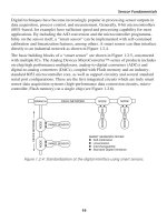
Figure 4.1.3: The Wheatstone bridge.
Sensor Signal Conditioning
33
A bridge measures resistance indirectly by comparison with a similar resistance. The
two principal ways of operating a bridge are as a null detector or as a device that
reads a difference directly as voltage.
When R1/R4 = R2/R3, the resistance bridge is at a null, regardless of the mode of
excitation (current or voltage, AC or DC), the magnitude of excitation, the mode of
readout (current or voltage), or the impedance of the detector. Therefore, if the ratio
of R2/R3 is fixed at K, a null is achieved when R1 = K
·
R4. If R1 is unknown and R4
is an accurately determined variable resistance, the magnitude of R1 can be found by
adjusting R4 until null is achieved. Conversely, in sensor-type measurements, R4 may
be a fixed reference, and a null occurs when the magnitude of the external variable
(strain, temperature, etc.) is such that R1 = K
·
R4.
Null measurements are principally used in feedback systems involving electrome-
chanical and/or human elements. Such systems seek to force the active element (strain
gage, RTD, thermistor, etc.) to balance the bridge by influencing the parameter being
measured.
For the majority of sensor applications employing bridges, however, the deviation of
one or more resistors in a bridge from an initial value is measured as an indication of

the magnitude (or a change) in the measured variable. In this case, the output voltage
change is an indication of the resistance change. Because very small resistance chang-
es are common, the output voltage change may be as small as tens of millivolts, even
with V
B
= 10 V (a typical excitation voltage for a load cell application).
In many bridge applications, there may be two, or even four, elements that vary.
Figure 4.1.4 shows the four commonly used bridges suitable for sensor applications
and the corresponding
equations which relate
the bridge output voltage
to the excitation voltage
and the bridge resistance
values. In this case, we
assume a constant voltage
drive, VB. Note that since
the bridge output is direct-
ly proportional to VB, the
measurement accuracy can
be no better than that of the
accuracy of the excitation
voltage.
Figure 4.1.4: Output voltage and linearity error
for constant voltage drive bridge configurations.
Chapter 4
34
In each case, the value of the fixed bridge resistor, R, is chosen to be equal to the
nominal value of the variable resistor(s). The deviation of the variable resistor(s)
about the nominal value is proportional to the quantity being measured, such as strain
(in the case of a strain gage) or temperature (in the case of an RTD).

The sensitivity of a bridge is the ratio of the maximum expected change in the output
voltage to the excitation voltage. For instance, if V
B
= 10 V, and the full-scale bridge
output is 10 mV, then the sensitivity is 1 mV/V.
The single-element varying bridge is most suited for temperature sensing using RTDs
or thermistors. This configuration is also used with a single resistive strain gage. All the
resistances are nominally equal, but one of them (the sensor) is variable by an amount
∆R. As the equation indicates, the relationship between the bridge output and ∆R is not
linear. For example, if R = 100 Ω, and ∆R = 0.152, (0.1% change in resistance), the out-
put of the bridge is 2.49875 mV for V
B
= 10 V. The error is 2.50000 mV – 2.49875 mV, or
0.00125 mV. Converting this to a percent of full scale by dividing by 2.5 mV yields an
end-point linearity error in percent of approximately 0.05%. (Bridge end-point linear-
ity error is calculated as the worst error in % FS from a straight line which connects the
origin and the end point at FS, i.e. the FS gain error is not included). If ∆R = 1 Ω (1%
change in resistance), the output of the bridge is 24.8756 mV, representing an end-point
linearity error of approximately 0.5%. The end-point linearity error of the single-ele-
ment bridge can be expressed in equation form:
Single-Element Varying Bridge End-Point Linearity Error ≈ % Change in Resistance ÷ 2
It should be noted that the above nonlinearity refers to the nonlinearity of the bridge
itself and not the sensor. In practice, most sensors exhibit a certain amount of their
own nonlinearity which must be accounted for in the final measurement.
In some applications, the bridge nonlinearity may be acceptable, but there are various
methods available to linearize bridges. Since there is a fixed relationship between the
bridge resistance change and its output (shown in the equations), software can be used
to remove the linearity error in digital systems. Circuit techniques can also be used to
linearize the bridge output directly, and these will be discussed shortly.
There are two possibilities to consider in the case of the two-element varying bridge.

In the first, Case (1), both elements change in the same direction, such as two identi-
cal strain gages mounted adjacent to each other with their axes in parallel.
The nonlinearity is the same as that of the single-element varying bridge, however
the gain is twice that of the single-element varying bridge. The two-element varying
bridge is commonly found in pressure sensors and flow meter systems.
Sensor Signal Conditioning
35
A second configuration of the two-element varying bridge, Case (2), requires two
identical elements that vary in opposite directions. This could correspond to two
identical strain gages: one mounted on top of a flexing surface, and one on the bot-
tom. Note that this configuration is linear, and like two-element Case (1), has twice
the gain of the single-element configuration. Another way to view this configuration is
to consider the terms R + ∆R and R – ∆R as comprising the two sections of a center-
tapped potentiometer.
The all-element varying bridge produces the most signal for a given resistance change
and is inherently linear. It is an industry-standard configuration for load cells which
are constructed from four identical strain gages.
Bridges may also be driven from constant current sources as shown in Figure 4.1.5.
Current drive, although not as popular as voltage drive, has an advantage when the
bridge is located re-
motely from the source
of excitation because the
wiring resistance does
not introduce errors in
the measurement. Note
also that with constant
current excitation, all
configurations are linear
with the exception of the
single-element varying

case.
In summary, there are
many design issues re-
lating to bridge circuits.
After selecting the basic configuration, the excitation method must be determined.
The value of the excitation voltage or current must first be determined. Recall that the
full scale bridge output is directly proportional to the excitation voltage (or current).
Typical bridge sensitivities are 1 mV/V to 10 mV/V. Although large excitation volt-
ages yield proportionally larger full scale output voltages, they also result in higher
power dissipation and the possibility of sensor resistor self-heating errors. On the
other hand, low values of excitation voltage require more gain in the conditioning
circuits and increase the sensitivity to noise.
Figure 4.1.5: Output voltage and linearity error
for constant current drive bridge configurations.
Chapter 4
36
Figure 4.1.7: Using a single op amp as a bridge
amplifier for a single-element varying bridge.
Figure 4.1.6: Bridge considerations.
Regardless of its value, the stability of
the excitation voltage or current directly
affects the overall accuracy of the bridge
output. Stable references and/or ratiometric
techniques are required to maintain desired
accuracy.
Amplifying and Linearizing Bridge
Outputs
The output of a single-element varying
bridge may be amplified by a single preci-
sion op-amp connected in the inverting

mode as shown in Figure 4.1.7.
This circuit, although simple,
has poor gain accuracy and also
unbalances the bridge due to load-
ing from RF and the op amp bias
current. The RF resistors must
be carefully chosen and matched
to maximize the common mode
rejection (CMR). Also it is dif-
ficult to maximize the CMR while
at the same time allowing dif-
ferent gain options. In addition,
the output is nonlinear. The key
redeeming feature of the circuit is
that it is capable of single supply
operation and requires a single op
amp. Note that the RF resistor connected to the non-inverting input is returned to V
S
/2
(rather than ground) so that both positive and negative values of ∆R can be accommo-
dated, and the op amp output is referenced to V
S
/2.
A much better approach is to use an instrumentation amplifier (in-amp) as shown
in Figure 4.1.8. This efficient circuit provides better gain accuracy (usually set with
a single resistor, RG) and does not unbalance the bridge. Excellent common mode
rejection can be achieved with modern in-amps. Due to the bridge’s intrinsic charac-
teristics, the output is nonlinear, but this can be corrected in the software (assuming
that the in-amp output is digitized using an analog-to-digital converter and followed
by a microcontroller or microprocessor).

Sensor Signal Conditioning
37
Various techniques are avail-
able to linearize bridges, but it
is important to distinguish be-
tween the linearity of the bridge
equation and the linearity of the
sensor response to the phenom-
enon being sensed. For example,
if the active element is an RTD,
the bridge used to implement the
measurement might have perfectly
adequate linearity; yet the output
could still be nonlinear due to the
RTD’s nonlinearity. Manufactur-
ers of sensors employing bridges
address the nonlinearity issue in a variety of ways, including keeping the resistive
swings in the bridge small, shaping complementary nonlinear response into the active
elements of the bridge, using resistive trims for first-order corrections, and others.
Figure 4.1.9 shows a single-element varying active bridge in which an op amp pro-
duces a forced null, by adding a voltage in series with the variable arm. That voltage
is equal in magnitude and opposite in polarity to the incremental voltage across the
varying element and is linear with ∆R. Since it is an op amp output, it can be used as
a low impedance output point for the bridge measurement. This active bridge has a
gain of two over the standard single-element varying bridge, and the output is linear,
even for large values of ∆R. Because of the small output signal, this bridge must usu-
ally be followed by a second amplifier.
The amplifier used in this circuit re-
quires dual supplies because its output
must go negative.

Figure 4.1.8: Using an instrumentation amplifier
with a single-element varying bridge.
Figure 4.1.9: Linearizing a single-element
varying bridge method 1.
Chapter 4
38
Another circuit for linearizing a single-
element varying bridge is shown in
Figure 4.1.10. The bottom of the bridge
is driven by an op amp, which main-
tains a constant current in the varying
resistance element. The output signal
is taken from the right hand leg of the
bridge and amplified by a non-inverting
op amp. The output is linear, but the cir-
cuit requires two op amps which must
operate on dual supplies. In addition,
R1 and R2 must be matched for accu-
rate gain.
A circuit for linearizing a voltage-driven two-element varying bridge is shown in Fig-
ure 4.1.11. This circuit is similar to Figure 4.1.9 and has twice the sensitivity. A dual
supply op amp is required. Additional gain may be necessary.
Figure 4.1.10: Linearizing a single-
element varying bridge method 2.
The two-element varying bridge circuit in Figure 4.1.12 uses an op amp, a sense resis-
tor, and a voltage reference to maintain a constant current through the bridge
(I
B
= V
REF

/R
SENSE
).

The current through each leg of the bridge remains constant (I
B
/2) as the resistances
change; therefore the output is a linear function of ∆R. An instrumentation amplifier
provides the additional gain. This circuit can be operated on a single supply with the
proper choice of amplifiers and signal levels.
Figure 4.1.11: Linearizing a two-element
varying bridge method 1 (constant
voltage drive).
Sensor Signal Conditioning
39
Figure 4.1.12: Linearizing a two-
element varying bridge method 2
(constant voltage drive).
Driving Bridges
Wiring resistance and noise pickup are the biggest problems associated with remotely
located bridges. Figure 4.1.13 shows a 350 Ω strain gage which is connected to the
rest of the bridge circuit by 100 feet of 30 gage twisted pair copper wire. The resis-
tance of the wire at 25°C
is 0.105 Ω/ft, or 10.5 Ω
for 100ft. The total lead
resistance in series with
the 350 Ω strain gage
is therefore 21 Ω. The
temperature coefficient
of the copper wire is

0.385%/°C. Now we will
calculate the gain and
offset error in the bridge
output due to a +10°C
temperature rise in the
cable. These calcula-
tions are easy to make,
because the bridge output voltage is simply the difference between the output of two
voltage dividers, each driven from a +10 V source.
The full-scale variation of the strain gage resistance (with flex) above its nominal
350 Ω value is +1% (+3.5 Ω), corresponding to a full-scale strain gage resistance of
353.5 Ω, which causes a bridge output voltage of +23.45 mV. Notice that the addi-
tion of the 21 Ω R
COMP
resistor compensates for the wiring resistance and balances the
bridge when the strain gage resistance is 350 Ω. Without R
COMP
, the bridge would have
Figure 4.1.13: Errors produced by wiring resistance
for remote resistive bridge sensor.